Geographical Diagram
The Tool is capable of displaying the geographical locations of power system resources on a map or a blank background based on the ENTSO-E Geographical Profile, which is derived from IEC 61968-Part 13. The major difference between two profiles is that each Location is uniquely associated with one PowerSystemResource in ENTSO-E Geographical Profile. If you have geographical information, but not in CIM format, you can import the geographical information in a user-defined format.
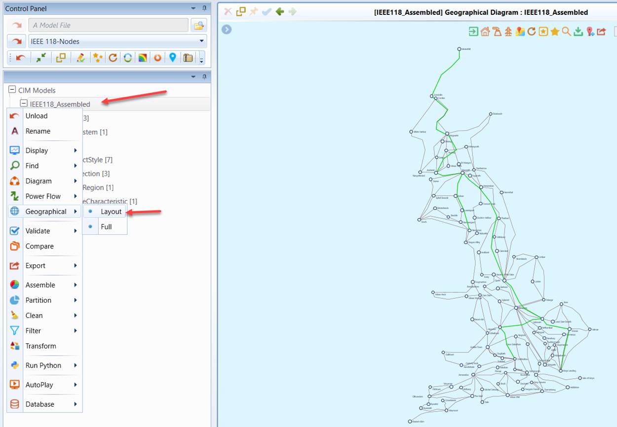
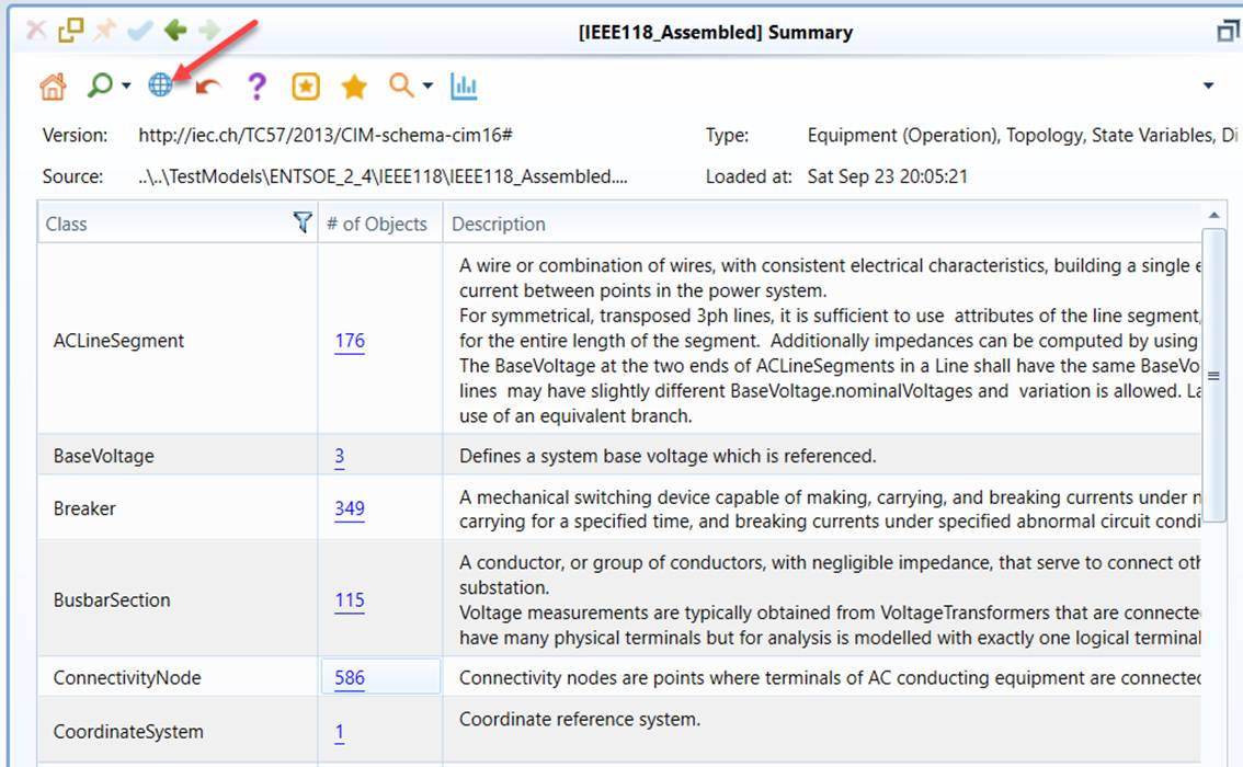
Geographical Diagrams are only available for any models that contain the Geographical data groups. Some of the interactive features, such as flow animations, are only available for the merged model which contains the information required to enable these features. For example, to display the power flow on the geographical diagram, the State Variable information (i.e. the power flow results) must be contained in the merged model. The Geographical Diagram can be called from the context menu associated with the model tree item or via the icon in the Quick Access Toolbar, as illustrated below. The Tool comes with a sample IEEE 118-Node model which contains both geographical information and solved power flow results. The Tool was pre-configured to enable users to load this sample model from the data source dropdown list. Users are encouraged to try this sample model to gain some hand-on experience.
The geographical diagram can be displayed on the supported maps. Users can enable this feature by turning on “Show Map Background” using one of the three approaches, as illustrated below.
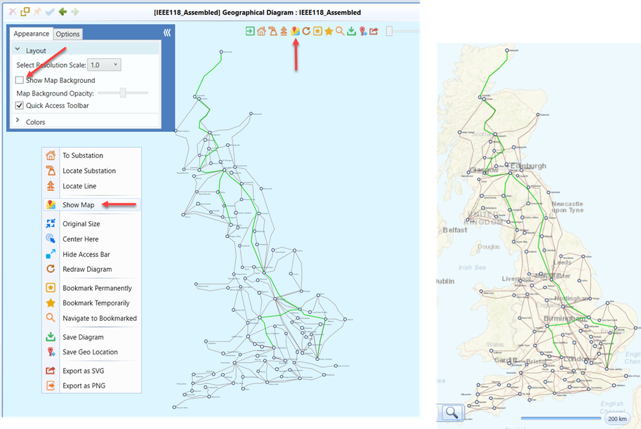
Without using map as background, the Tool is still capable of displaying the geographical diagram in a blank background. The displayed geographical diagram is basically identical to the one displayed on the map.
Navigations between Geographical Diagram and Other Displays
The Geographical Diagram is seamlessly integrated with the schematic diagrams including Substation Diagram and Neighborhood Diagram. Users can overview the diagram of the selected substation through a popup by hovering the mouse over the substation graphical symbol on a Geographical Display or navigate to the Substation Diagram/Neighborhood Diagram through a context menu associated with the substation graphical symbol on a Geographical Display.
Similarly, users can also navigate from the schematic diagrams to the geographical diagrams through the context menu in the schematic diagrams, as illustrated below.
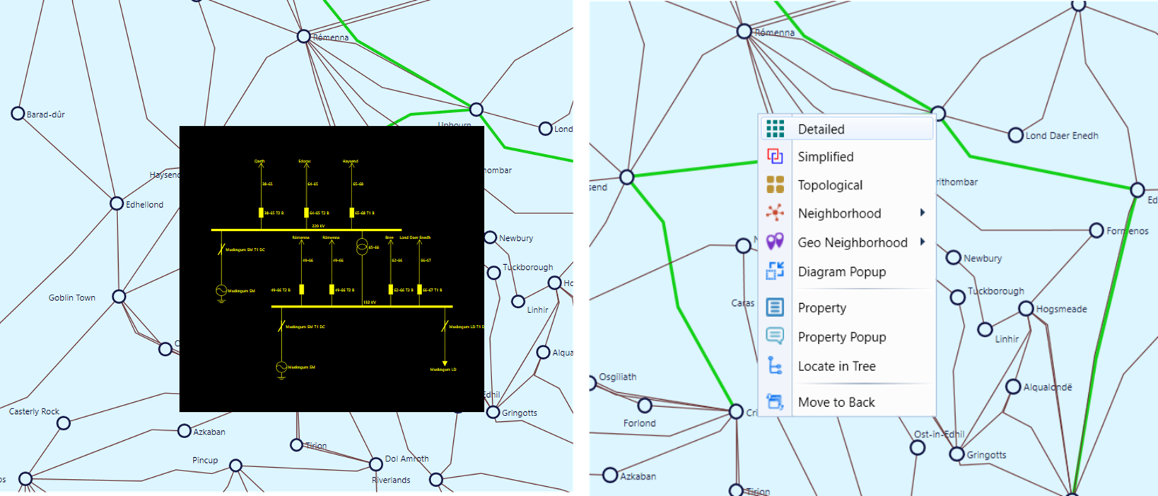
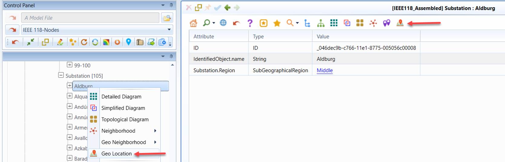
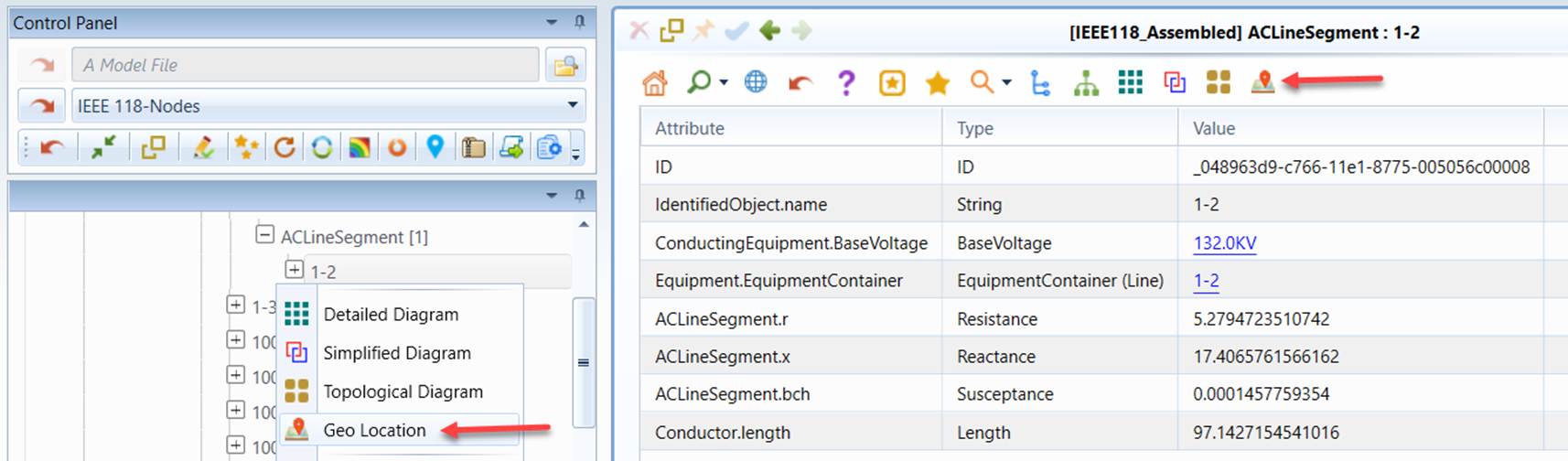
Navigations between geographical diagrams and other displays are also supported, as illustrated below. Users can navigate from a Substation/ACLineSegment Form Display to a Geographical Diagram with the selected Substation/ACLineSegment highlighted. The same type of navigation is also provided for the Substation/ACLineSegment tree items in the Navigation Tree. Users can also navigate from the geographical diagram to the corresponding Form Display through the “property” context menu item as shown above.
Note
The “Geo Location” navigation is data-driven. If Substations/ACLineSegments have no geo locations associated in the model, the “Geo Location” context menu items or hyperlinks will not be available for these Substations/ACLineSegments.
Calling Substation Diagrams from Geographical Diagram
While navigations are provided between Geographical Diagram and Substation Diagram, users may want to call Substation Diagram directly from Geographical Diagram through a popup Window. This feature will allow users to drill down into a Substation from Geographical Diagram without losing the context. The Substation Diagram can be called from Geographical Diagram in the following two ways:
- Double-click the graphical symbol or label of the selected Substation
- Right-mouse-click the graphical symbol or label of the selected Substation and select Substation Popup
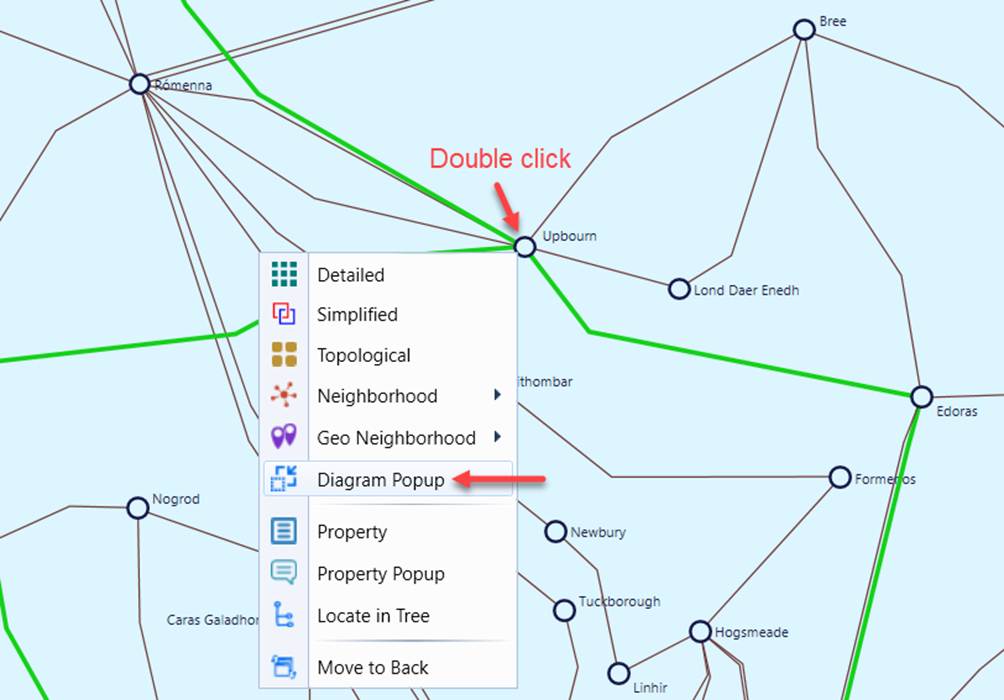
Once invoked, a separate Windows will pop up on top of the current Geographical Diagram to display the default type of the Substation Diagrams (typically the Detailed Substation Diagram). Users can always change the type of the Substation Diagrams using context menu, as illustrated.
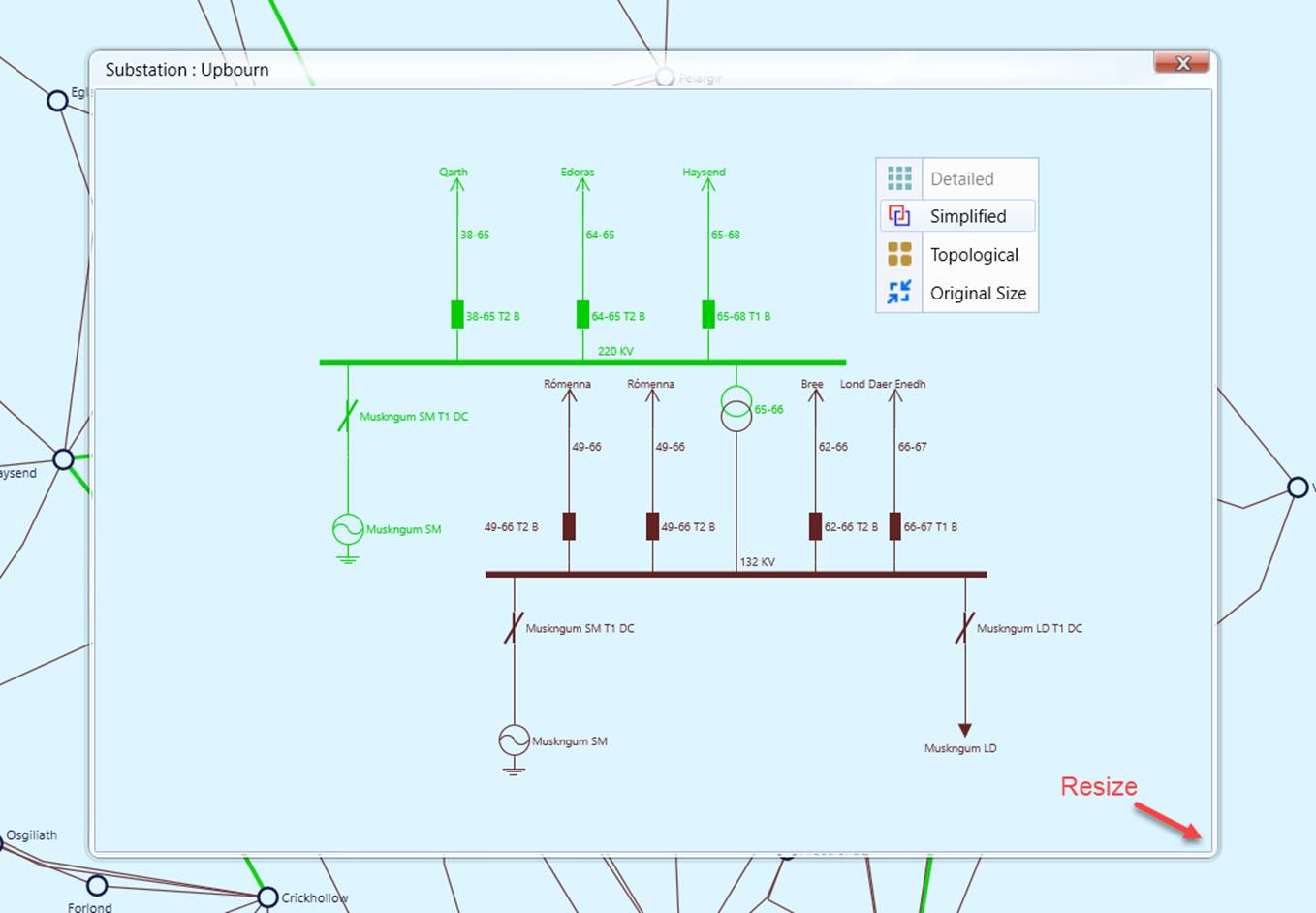
A popup Substation Diagram is just like a typical Substation Diagram in appearance. It inherits all of the current user preference settings. Users can also zoom and pan the diagrams in a popup Substation diagram. But there are some limitations or restrictions in functionality and navigation. For example, the popup Substation Diagram is read only. The only navigation link provided in a popup Substation Diagram is to the neighboring substations via double-clicking of the selected symbol/label representing neighboring substations. The popup Window can be resized by dragging the line crossing the bottom-right corner, as illustrated above. It can be closed by clicking the “x” icon at the top-right corner.
Popup Substation Diagrams can also be invoked from schematic or geographical Neighborhood Diagram.
Regional Geographical Diagram
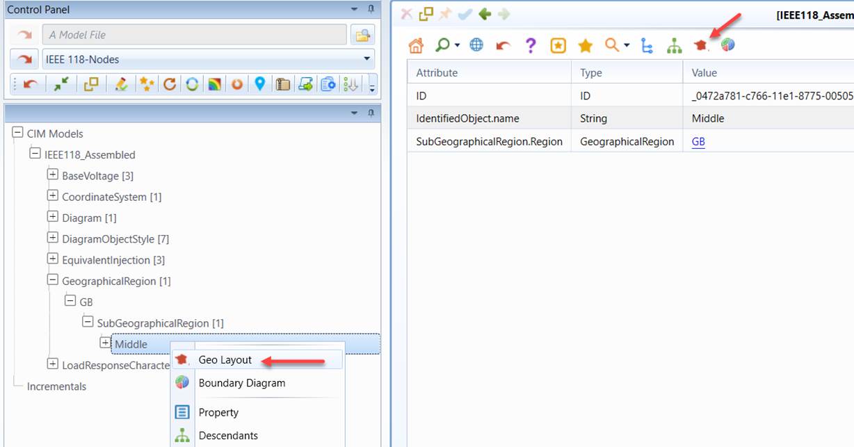
When calling the Geographical Diagram from the mechanisms, the entire Geographical Diagram will be displayed. Alternatively, users can also choose to display a regional Geographical Diagram from the menu items associated with the selected GeographicalRegion or SubGeographicalRegion in the Navigation Tree or the corresponding Command Icon from the related Object Form, as illustrated below. A regional Geographical Diagram only shows Substation/Lines belonging to this particular region.
Partial Geographical Diagram
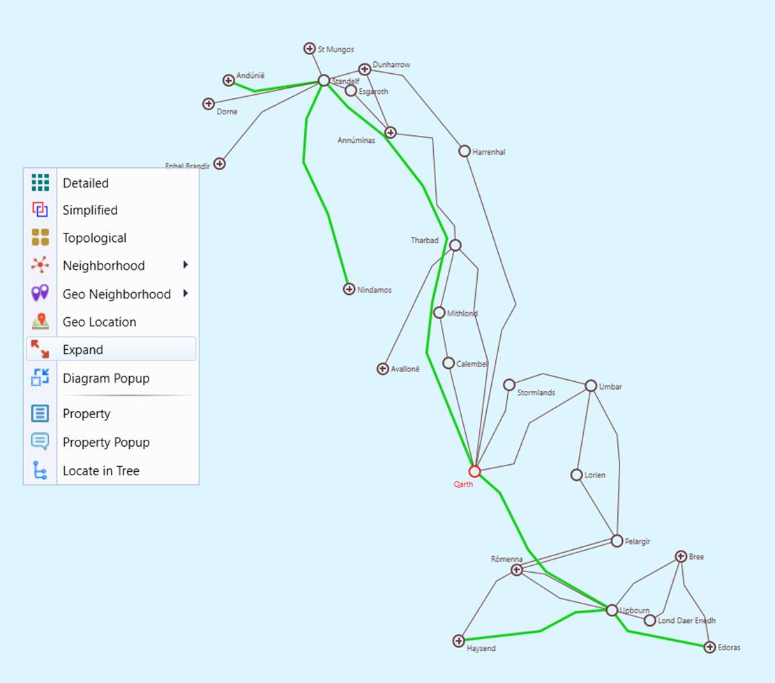
Users can display a portion of the geo diagram form a selected Substation as geo neighborhood diagram, which layout a selected substation and its neighboring Substations/Lines according to their geographical information. User can also expand the geo neighborhood diagram to create a partial geographical diagram and save it for the future use, as illustrated below.
Note
The “Geo Neighborhood” navigation is data-driven. If Substations/ACLineSegments have no geo locations associated in the model, the “Geo Neighborhood” context menu items or hyperlinks will not be available for these Substations/ACLineSegments.
Visualization of Regions in a Geographical Diagram
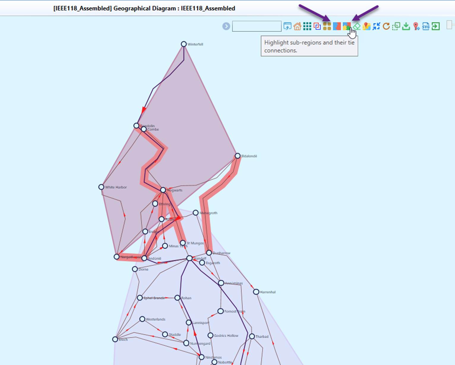
The Tool allows users to visualize regions (GeographicalRegion or SubGeographicalRegion) within a geographical diagram, as illustrated below. Once enabled, a colored polygon overlay is generated for each region, highlighting the geographical area it covers. Additionally, tie-lines connecting different regions are also highlighted, providing a clear representation of interconnections.
Layout of Geographical Diagram with Missing or Erroneous Geographical Information
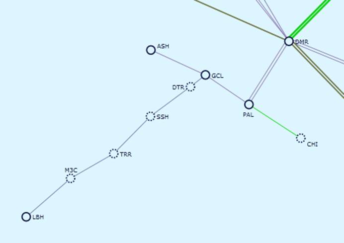
When only partial geographical information is available, the network topology information will be used to fill the gap. For example, if there is no geographical information for transmission lines, the network connectivity information will be used to draw straight lines between stations. Similarly, if a station doesn’t have geographical information, it will be placed based on the layout algorithm. In the following diagram, stations are connected by straight lines due to the lack of line geographical information and stations without geo information are shown in dotted circle. The resulting diagrams are called geo-schematic diagrams.
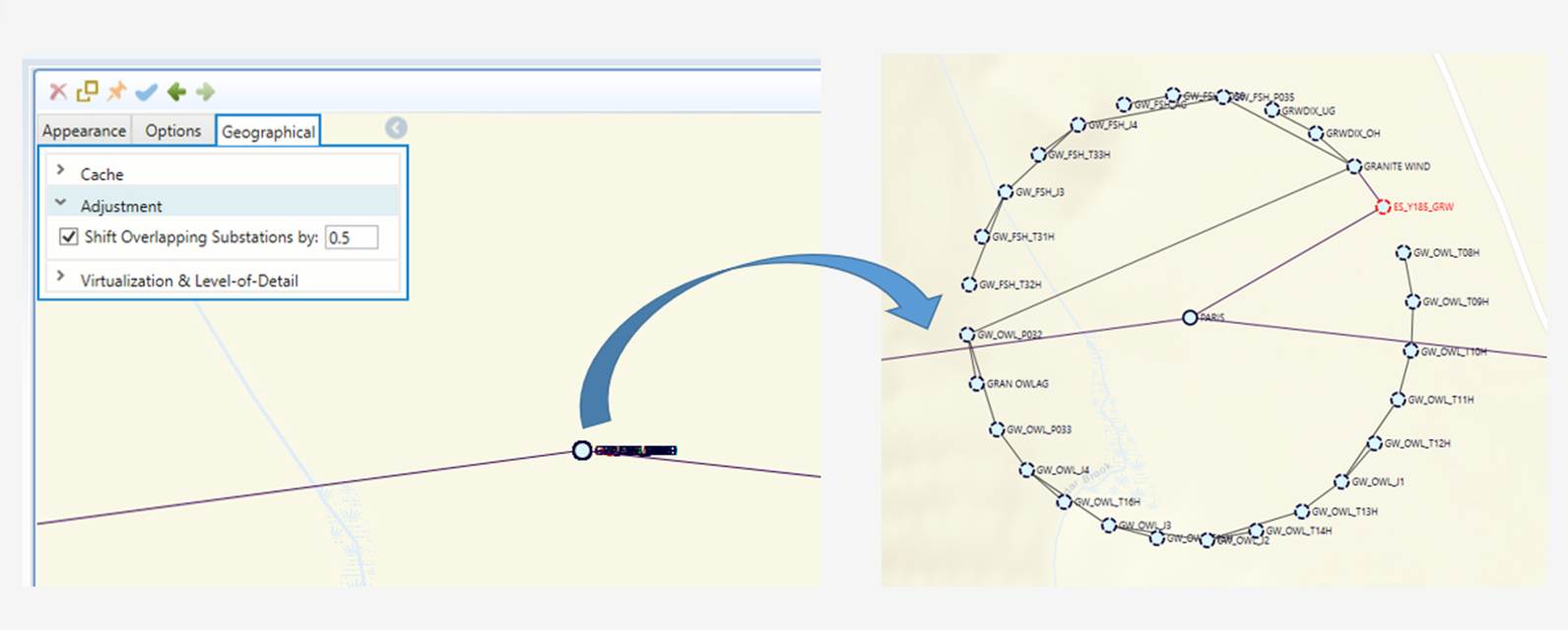
Some geographical data in the model may be inaccurate or imprecise. A common example is multiple substations sharing the same geographic coordinates, resulting in what are referred to as overlapping substations. When such cases are detected, the geo layout algorithm automatically adjusts their positions to ensure that their connections can be clearly displayed.
The original location of the master substation—typically the most highly meshed high-voltage substation—is preserved. The remaining overlapping substations are distributed around the master location using a spreading algorithm to improve visibility and readability. These repositioned substations are displayed with a dashed-circle to indicate that their positions are approximate rather than exact.
The radius of the spreading circle (in pixels) is configurable, allowing users to control the degree of separation. The sample below illustrates a group of overlapping substations distributed around a master substation within a radius of 0.5 pixels (approximately 100 feet).
Full Geo Layout
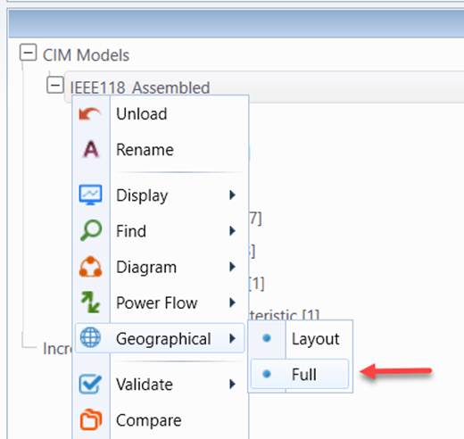
In many cases, the geographical information is unavailable for some regions (GeographicalRegion or SubGeographicalRegion), typically the external regions. By default, the line/substations of these regions will not be displayed in the geo diagram. Users, however, can explicitly request that all of the line/substations of any regions be displayed in the geo diagram. This is accomplished by invoking “Full Geo Layout” from the context menu associated with the model. The resulting geo diagrams are typically messy due to the fact that the many line/substations of the external regions don’t have geographical information. This feature, however, makes it possible for users to manually build a portion of the geo diagram by dragging and dropping the Substation symbols and then saving the adjusted geo diagram.
Multi-Station Diagram
A Multi-Station Diagram can be generated from a Geographical diagram, full or partial, showing the detailed network information.
Rendering of Large Geographical Diagrams
For large-scale Geographical Diagrams, rendering can be time-consuming and resource-intensive, especially when handling extensive network data. As the diagram size increases, the Tool must process a higher number of elements, including substations, transmission lines, and labels, which can lead to performance bottlenecks. This challenge is particularly noticeable when zooming, panning, or making adjustments to the diagram.
To address this, optimization techniques including Diagram Virtualization and Level-of-Detail adjustments can be applied to enhance performance while maintaining clarity and usability. These methods ensure that only the necessary portions of the diagram are processed at any given time, significantly improving responsiveness and efficiency.
Reduction of Geo Data Size
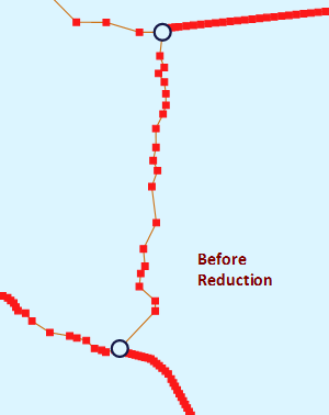
If your geo data come from GIS, they may contain very detailed geo information, including locations of transmission towers. Such detailed geo information may create a performance burden for geo diagram rendering. The Tool provides users an option to reduce the size of the imported geo data before rendering the geographical diagram. When enabled, this function will combine the line geo locations to reduce the size of the imported geo data. Multiple segment positions may be combined as single line segment positions if they fit certain criteria, as illustrated below:
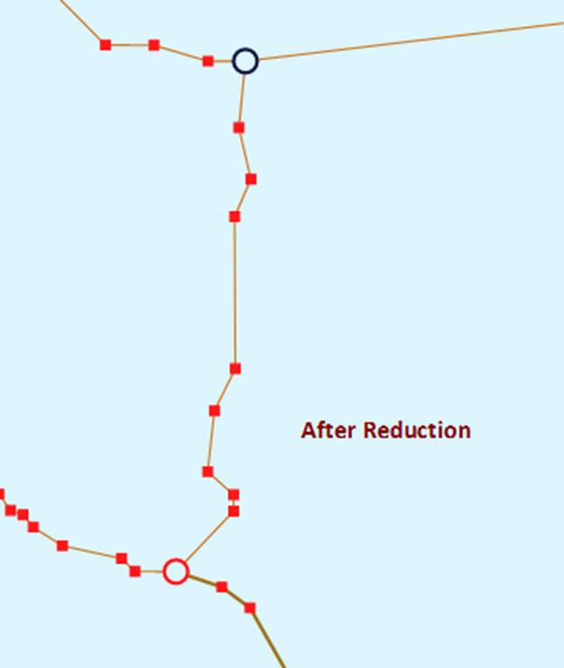
The geo reduction algorithm is controlled by a set of parameters specified in the GeoReductionConfig element of the configuration file, as shown below

Where
linePointReductionEnabled: If true, the algorithm will combine small line segments based on the criteria to reduce the number or line PositionPoints.minimumPointsToTriggerReduction: If number of line points exceed the specified minimum number and m_reduceGeoLinePoints is 'true', and the average point/line ratio exceeds minimumPointLocationRatioToTriggerReduction, the line segments will be reduced.minimumPointLocationRatioToTriggerReduction: if the average point/line ratio exceeds minimumPointLocationRatioToTriggerReduction, and number of line points exceed the specified minimum number and m_reduceGeoLinePoints is 'true', the line segments will be reduced.directLineConnection: if true, all location points on the lines will be ignored. Stations are connected by straight lines.angleTolerance: Minimum angle (in radian) used to straighten the sloped lines.straightLineTolerance: Maximum number of pixels used to straighten horizontial or vertical lines. If the Y or X of two points is below the specified maximum number of pixels, the two points will be adjusted as horizontal or vertical.equalPointTolerance: Coordinate overlap tolerance in both x and Y.multiLineAngleTolerance: Minimum angle (in radian) used to straighten the sloped multi-lines.multiLineStraightLineTolerance: Maximum number of pixels used to straighten horizontial or vertical multi-lines. If the Y or X of two points is below the specified maximum number of pixels, the two points will be adjusted as horizontal or vertical.multiLineEqualPointTolerance: Coordinate overlap tolerance in both x and Y for multi-lines.
Note geo reduction configuration is a global setting shared by all of the loaded models. It is also used for geo data import.
When geo reduction is enabled, multiple line segment may be combined in geographical diagram. However, users can still view the detailed geo locations of the same area by calling the geo neighborhood diagram.
Capture Capture1
Locating Substations/Lines on a Geographical Diagram
One of the major information searching mechanism supported in the Tool is visual information searching. It helps user find the useful information through visualization. In response to user’s request, the Tool auto-generates the diagram, zooms the generated diagram to a proper size, centers the identified object, and highlights it in different color.
To locate a Substation/Line:
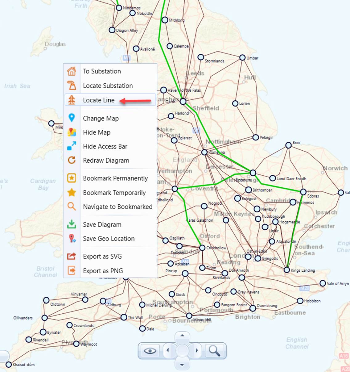
- Right-mouse-click a blank spot in the geographical diagram and select the “Locate Line” or “Locate Substation” context menu item, as illustrated below.
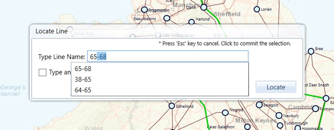
- An information search wizard will pop up. As users enter the name of the Substation/Line, the hint list will be updated. Typically, after enter 2 to 3 letters, users shall be able to find the name from the hint list.
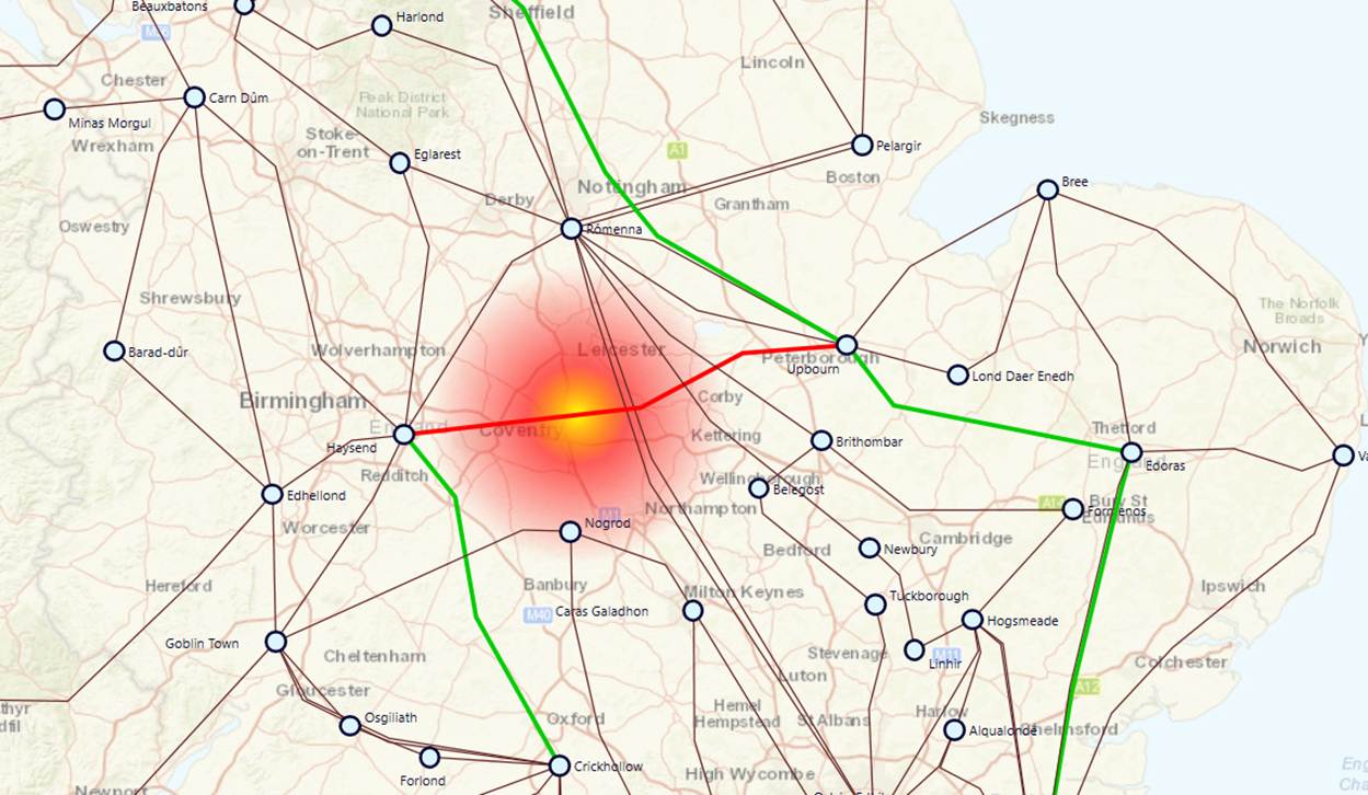
- Once the query is submitted, the Tool will zoom the generated diagram to a proper size, center the identified object, and highlights it in red color, as illustrated below.
.
Power Flow Visualization
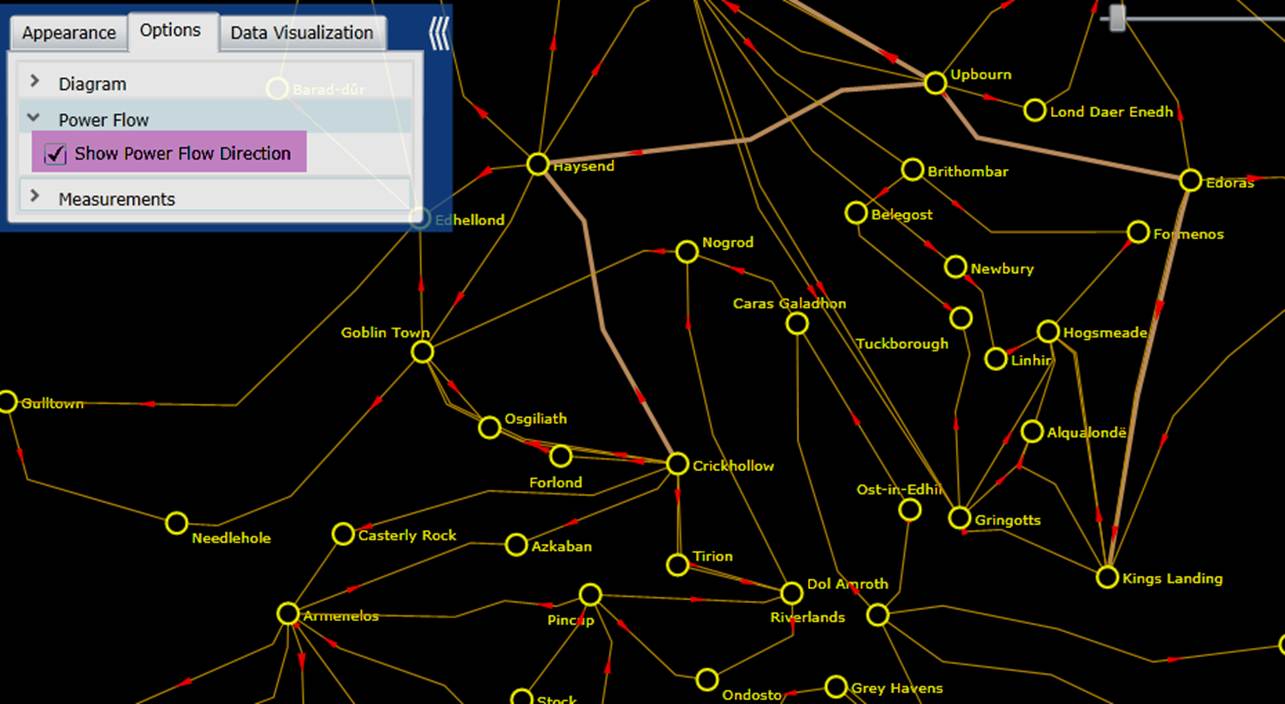
Users can also enable flow animations to visualize the power flow distribution on a geographical diagram. This feature is only available for a merged model that contains the State Variable data group. Once the “Show Power Flow Direction” checkbox is selected, the flow animation will be enabled in the geographical diagram. Additionally various data visualization techniques are applied to help users understand the data. For example, the size of the arrow that represents the power flow and its moving speed are determined by the apparent power of the branches. If an over-limiting condition is detected, the branch and its flow arrow will flash to alert users. But, in general, only minimum set power flow information can be displayed on a geographical diagram. This is a designed behavior, aimed at avoiding “information overload’. To check the detailed power flow results, users shall navigate to the corresponding schematic diagrams for details.
Backbone Visualization
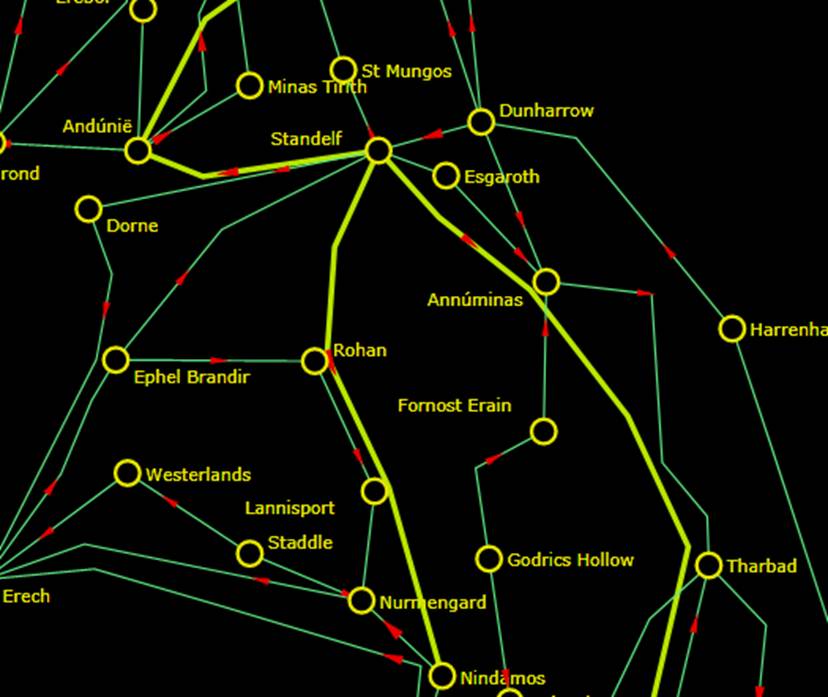
In a geographical diagram, high voltage backbone transmission lines can be visually highlighted. They are represented as thicker lines as shown below.
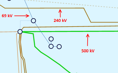
Transmission lines are classified into 3 groups: low-voltage (1 pixel), medium-voltage (2 pixels), and high-voltage (3 pixels). Users can define the kV range for each group in the Presentation Style definition, as shown below.

The 3 kV groups are defined as follows:
- Low-Voltage <= maxLowKV
- High-Voltage >= minHighKV
- ü Medium-Voltage > maxLowKV and Medium-Voltage < minHighKV
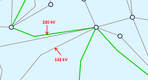
The three voltage levels are normally defiled in the default Presentation Style as shown above. Users, however, can overload the default settings by defining a special Presentation Style. The following example overloads the default voltage level settings. It basically specifies any transmission line above 140 kV shall be displayed as 3-pixel thick lines.

Display Options
The Tool provides a variety of options, enabling users to display/hide the information in a geographical diagram. The following screenshots illustrate what display options are available for a geographical diagram.
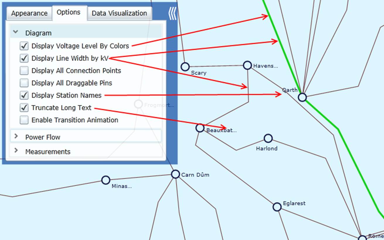
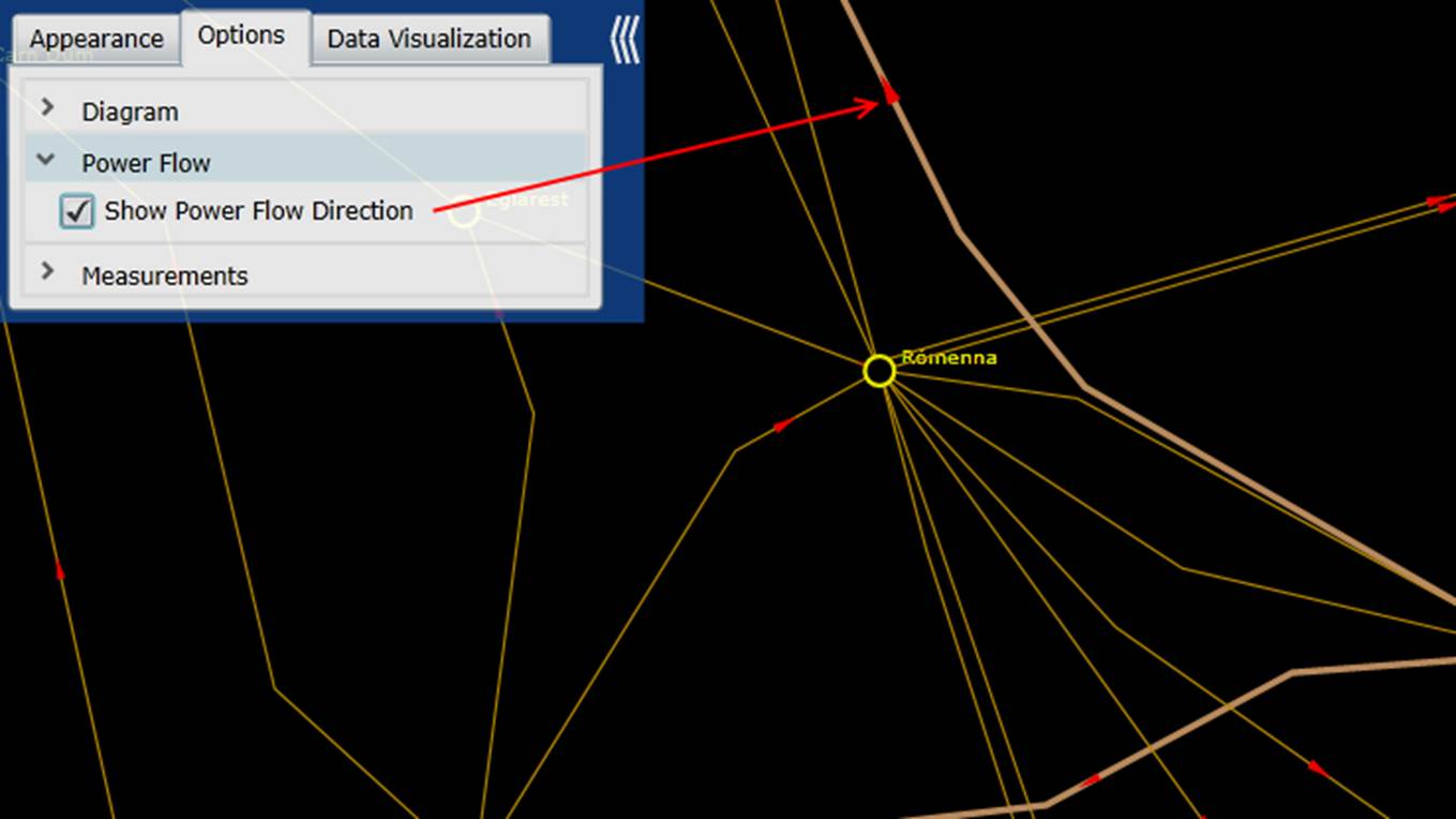
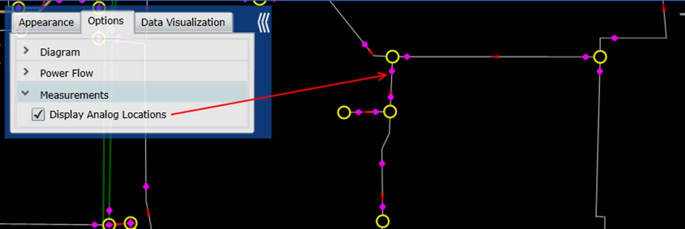
Resolution Adjustment
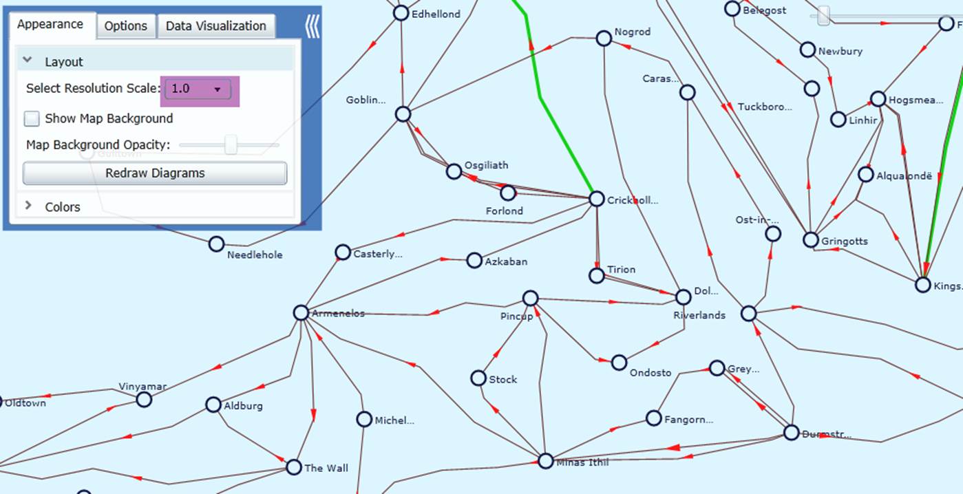
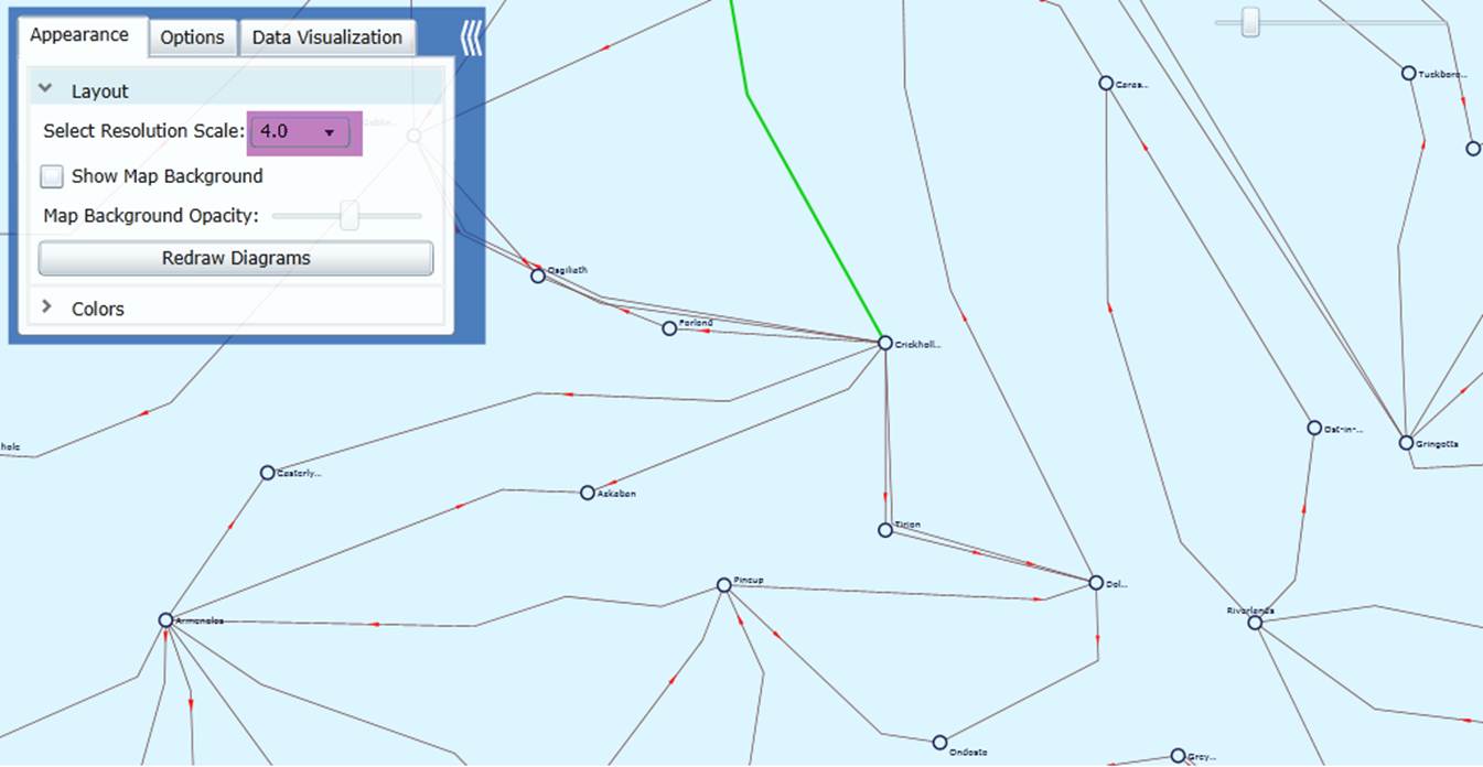
Layout of the geographical diagram is quite model-dependent. If the substations are located in small geographical area, the generated geographical diagram may not be very clear due to the overlapping of graphical symbols. In that case, users can adjust the Resolution Scale, as illustrated below. An increased resolution scale will spread the geographical diagram by using small graphical symbols. During zoom in/out, the graphical symbols and the connections will be dynamically adjusted to maintain the same size, thus resulting in fine resolutions. The 2nd diagram shows a fine-resolution counterpart of the 1st diagram after the resolution scale is raised from 1.0 to 4.0.
Option for Rendering Large Geographical Diagrams
Rendering performance for large geographical diagrams has been further improved through intelligent caching techniques. Geographical information is cached at the UI layer to avoid repeated retrieval from the backend, allowing previously rendered components to be reused efficiently. This approach is particularly effective because geographical data typically remains static during normal operation.
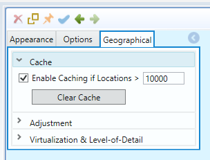
The caching mechanism is highly configurable, as illustrated below. Users can choose whether to enable caching and define the minimum number of Locations that will trigger it. Once the specified threshold is exceeded, caching is automatically applied to optimize rendering performance for large-scale diagrams.
Through multi-resolution rendering and intelligent caching, a geo diagram with approximately 65,000 substations now renders in about 10 seconds on first load and 5 seconds thereafter, delivering substantially improved responsiveness for large-scale network models.
Map Opacity Adjustment
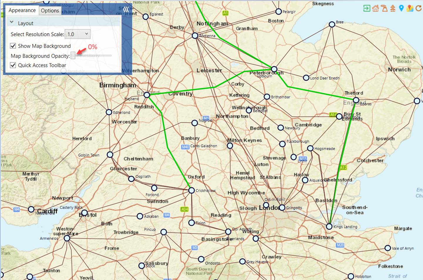
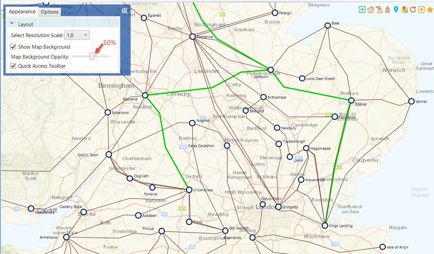
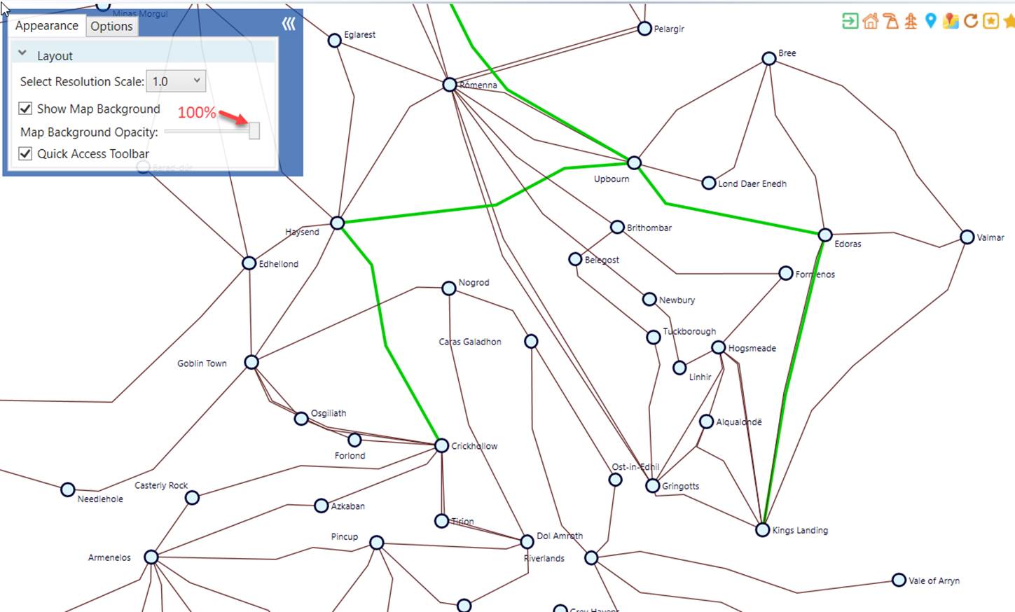
Map background can be noisy at times, especially containing lines and shapes similar to diagram components. An opacity mask slider can be used to completely show or hide the map background, or anywhere in between. The following screenshots demonstrate how map background can be faded when the opacity adjusted from 0 to 100%.
Tips
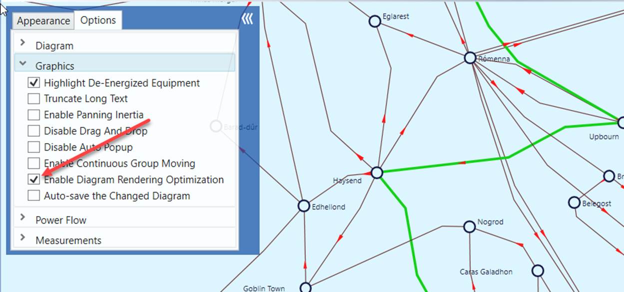
If your geographical diagram is large, there will be a performance issue. It takes long time to render a large diagram. This is due to the limitation of .NET graphical support. You can mitigate this issue by enabling diagram rendering optimization as illustrated below. When this option is enabled, some of the time-consuming graphical components, such as power flow animation, measurements, etc., will not be displayed for large diagrams. The ultimatum solution, however, is to support diagram virtualization in the future release.