Power Flow Tutorial
The best way to learn is hands-on. This tutorial is made up of 7 hands-on labs. It is expected that, after going through these labs, users will learn the basic and major features of power flow support. Before starting the labs, users must set up the environment.
Hands-On Lab 1: Running Power Flow for the First Time
- Objective: To learn how to run power flow and the basic.
- Test Model: Svedala, an assembled CGMES 3.0/CIM 17 model from ENTSO-E CGMES 3.0 Test Configurations (https://www.entsoe.eu/Documents/CIM_documents/Grid_Model_CIM/TestConfigurations_packageCASv2.0.zip). This is a node/breaker model containing reality-based Substations and with power flow results published.
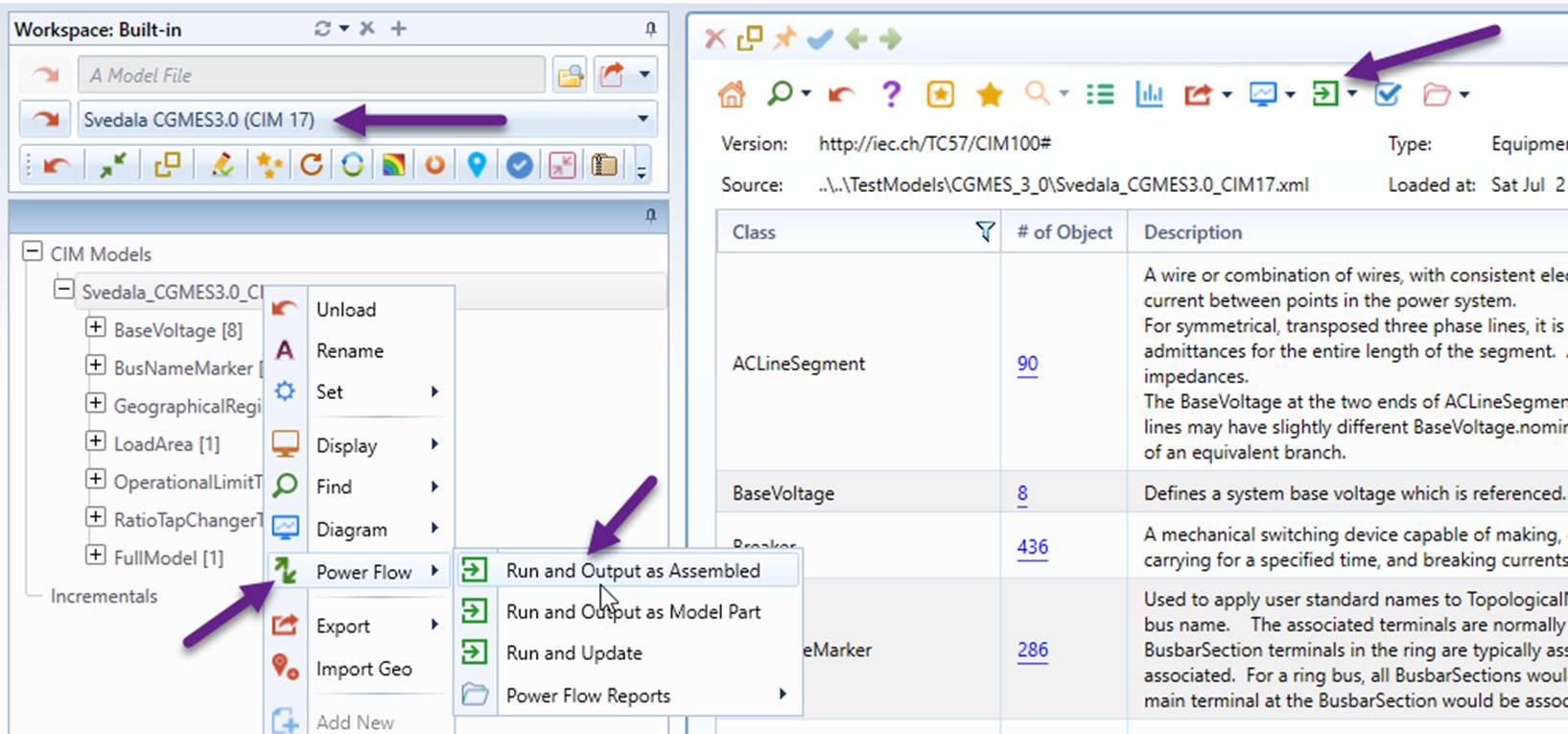
- Load “Svedala CGMES 3.0 (CIM 17)” from data source dropdown list, as illustrated.
- Invoke “Power Flow→Run and Output as Assembled” from the context menu associated with the model tree node or from the icon dropdown in the model Summary display, as illustrated
Note
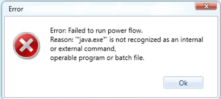
If you see the following message, it means that Java is not installed. The power flow engine, i.e. PowSyBl, is a java application. It requires Java 11 or a later version to be installed. Please Set Up Power Flow Environment first.
- After power flow execution is completed, a separate model is created with the calculated power flow results and a message box pops up, displaying execution status information. The Power Flow Summary Report is subsequently displayed, showing the statistic of the power flow results.
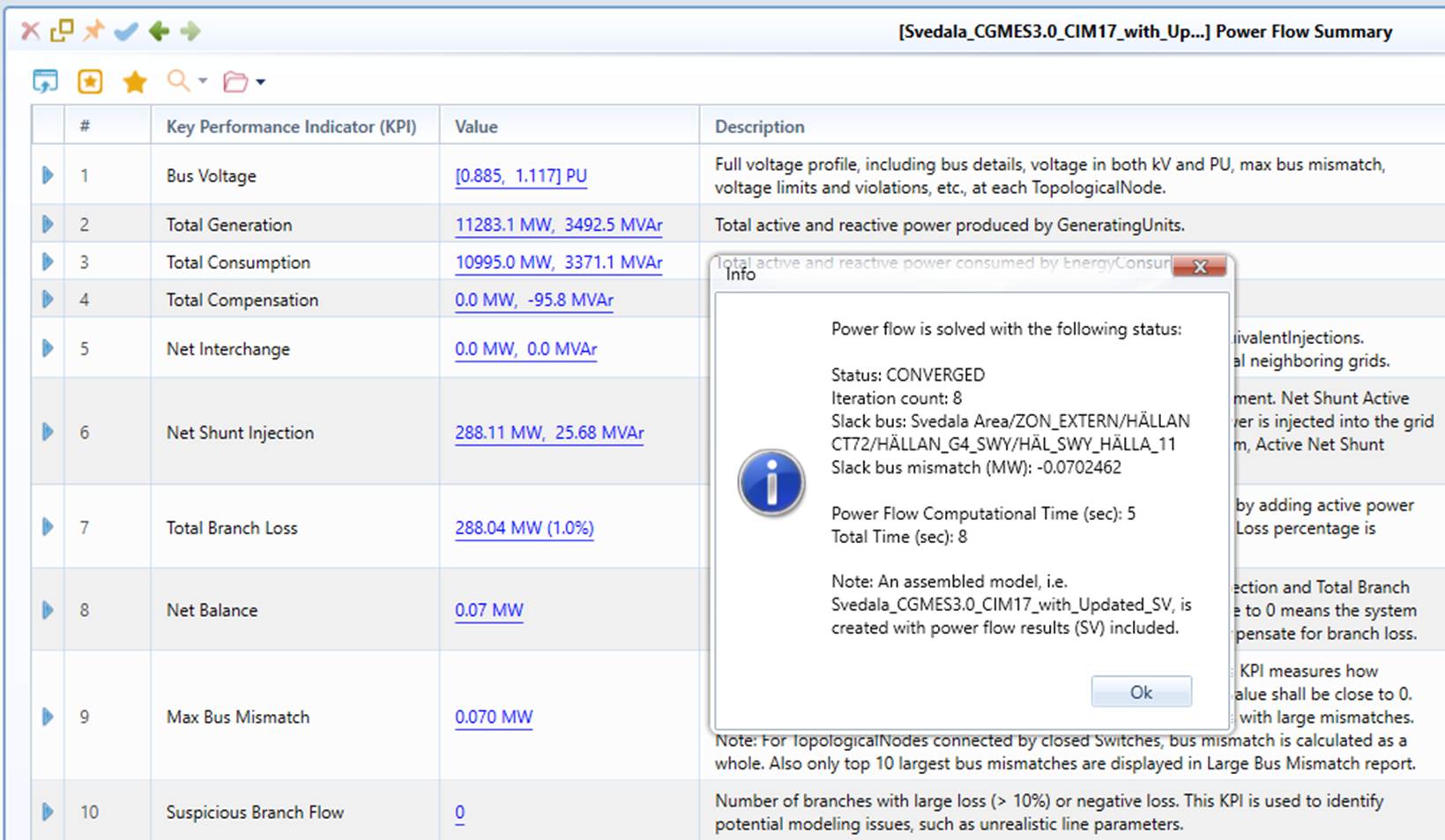
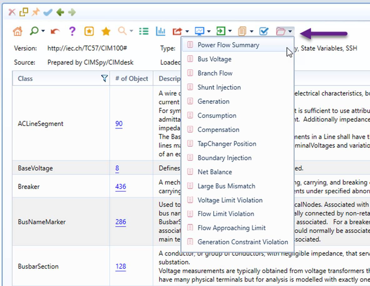
- The Power Flow Summary Report contains links to the detailed reports, which can also be called from the icon dropdown in the model summary display, as illustrated.
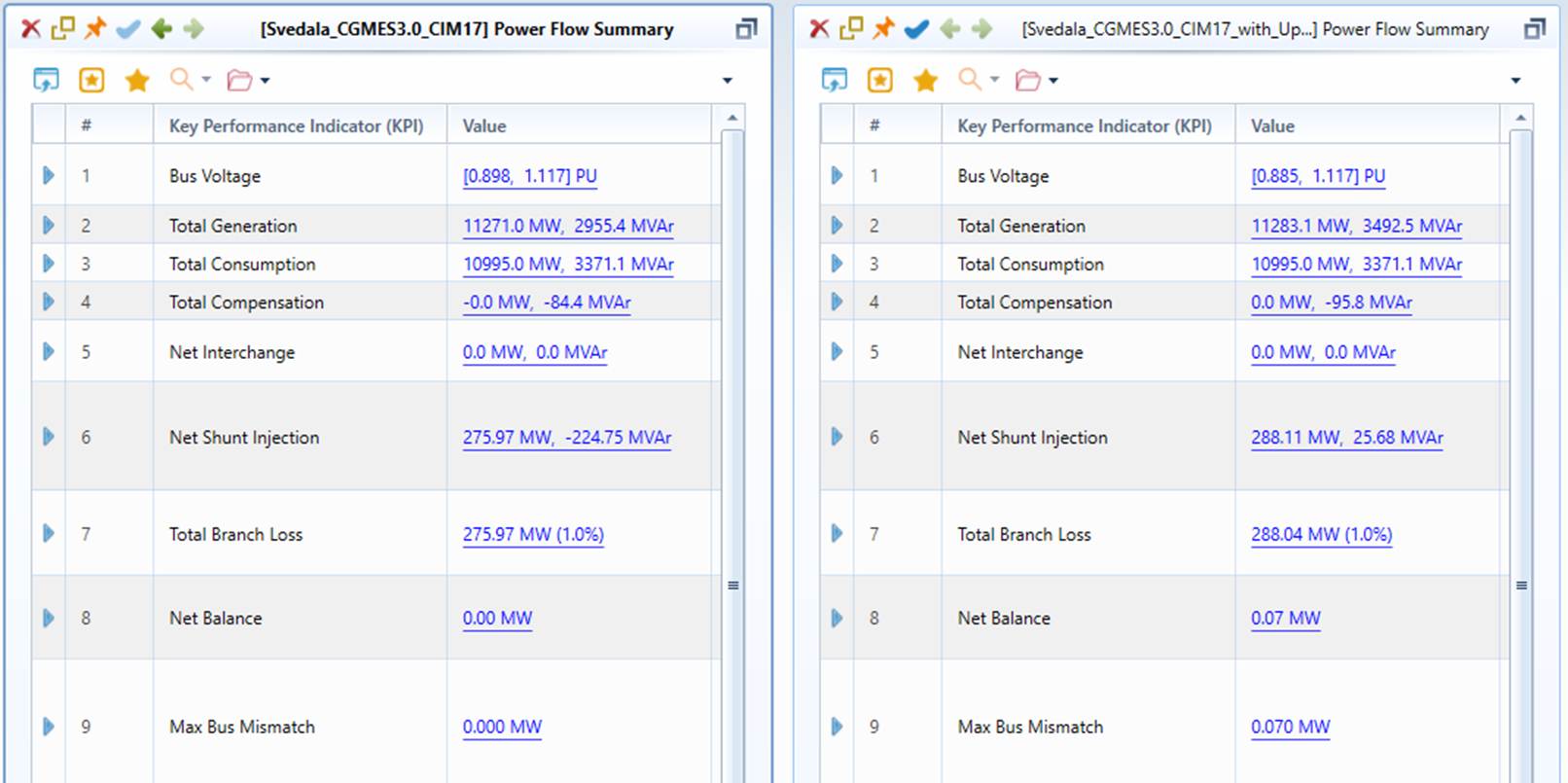
- Use the Split View to compare the calculated power results (right view) with those published (left view). The side-by-side Power Flow Summary Reports allows power flow results to be compared from different perspectives.
Tips: It is tricky to work with split views.
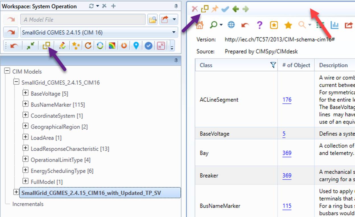
- Split view can be created from the command icons as illustrated below.
-
At any time, only Active view responds to users’ activities. Therefore, users must explicitly activate the intended view by clicking the title bar prior to any activities.
-
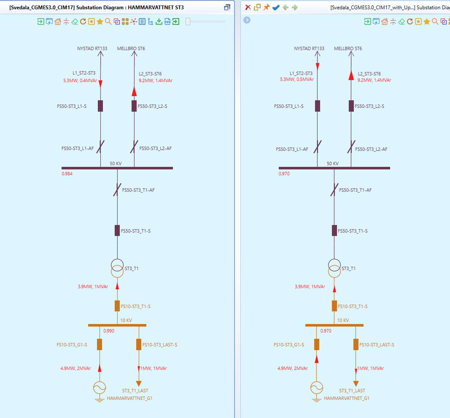
Use the split view to compare power flow results for a Substation. This can be achieved by displaying a Substation Diagram for the same Substation in the two models.
Hands-On Lab 2: Running Power Flow for IGM
- Objective: To learn how to run power flow for an Individual Grid Model (IGM). IGM is standardized model package submitted by Transmission System Operator (TSO) to ENTSO-E.
- Test Model: MicroGrid, a CGMES 2..4.15/CIM 16 IGM package from ENTSO-E CGMES 2.4.15 Test Configurations (https://www.entsoe.eu/Documents/CIM_documents/Grid_Model_CIM/CGMES_v2.4.15_TestConfigurations_v4.0.3.zip). This is a node/breaker model containing all model parts of an IGM & boundary, with power flow results published.
The test procedures are similar to Lab1, with the following notes:
- The Test Model can be loaded from the data source dropdown, as illustrated below:
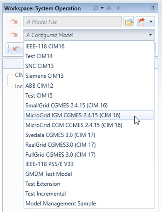
- Boundary set (i.e. EQ_BD/TP_BD) must be loaded to run power flow. IGM is not a complete dataset. It depends on boundary set.
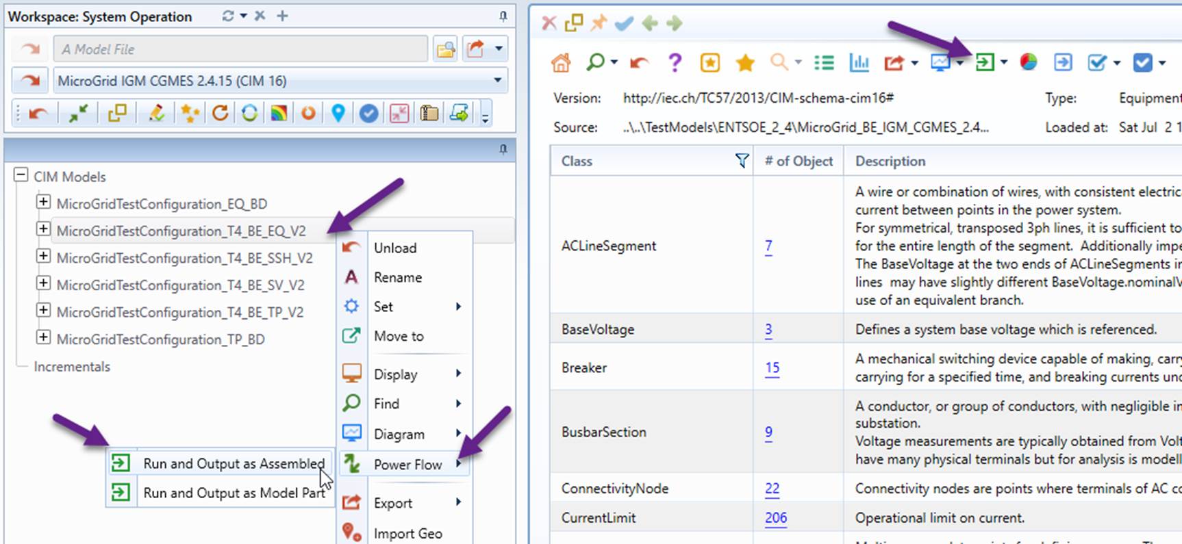
- Power flow execution can only be invoked from the Equipment (EQ) or Boundary Equipment (EQ_BD) model part, as illustrated. An assembled model can also be created from these model parts.
Hands-On Lab 3: Running Power Flow for CGM
- Objective: To learn how to run power flow for an Common Grid Model (CGM). CGM is model package merged from IGMs by ENTSO-E and shared with TSOs.
- Test Model: MicroGrid, a CGMES 2..4.15/CIM 16 IGM package from ENTSO-E CGMES 2.4.15 Test Configurations (https://www.entsoe.eu/Documents/CIM_documents/Grid_Model_CIM/CGMES_v2.4.15_TestConfigurations_v4.0.3.zip). This is a node/breaker model containing all model parts of two IGMs & boundary, and with power flow results published.
The test procedures are similar to Lab1, with the following notes:
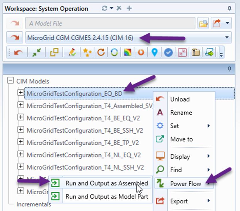
- The Test Model can be loaded from the data source dropdown, as illustrated below:
- Boundary set (i.e. EQ_BD/TP_BD) must be loaded to run power flow. IGMs are connected at boundary set.
- Power flow execution can only be invoked from the Boundary Equipment (EQ_BD) model part, as illustrated. An assembled CGM model can also be created from this model part.
Hands-On Lab 4: Running Power Flow for Reality-Based Large Model
- Objective: To test power flow with a large reality-based model.
- Test Model: RealGrid, an assembled CGMES 3.0/CIM 17 model from ENTSO-E CGMES 3.0 Test Configurations (https://www.entsoe.eu/Documents/CIM_documents/Grid_Model_CIM/TestConfigurations_packageCASv2.0.zip). This is a bus/branch model containing 6252 buses, based on reality, and with power flow results published.
The test procedures are similar to Lab1, with the following notes:
- The Test Model can be loaded from the data source dropdown, as illustrated below.
- The power flow execution status is shown below.
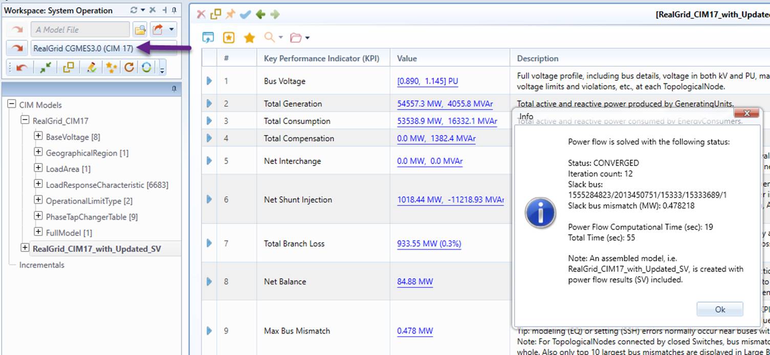
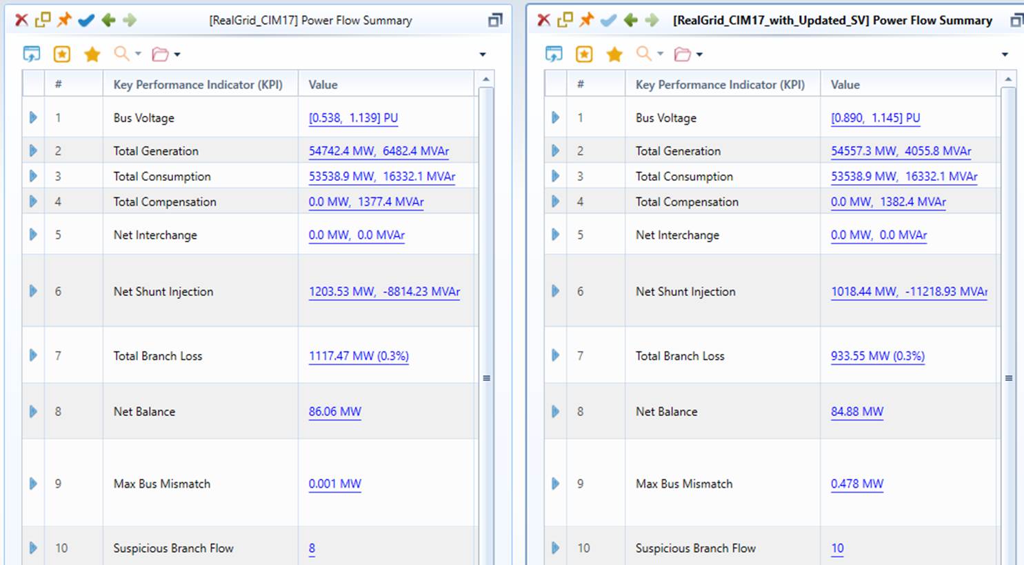
- The power flow comparison results are shown below: (left: published, right: calculated)
Hands-On Lab 5: Interactive Power Flow
- Objective: To learn how to run power flow in interactive mode.
- Test Model: SmallGrid, an assembled CGMES 2..4.15/CIM 16 IGM package from ENTSO-E CGMES 2.4.15 Test Configurations (https://www.entsoe.eu/Documents/CIM_documents/Grid_Model_CIM/CGMES_v2.4.15_TestConfigurations_v4.0.3.zip). This is a node/breaker model containing all model parts of an IGM & boundary and with power flow results published. However the Topology (TP) and State Variable (SV) model parts are removed. So the assembled test model contains the minimum data set required to run power flow, i.e. Equipment (EQ) and Steady State Hypothesis (SSH) model parts.
The Interactive Power Flow feature enables users to simulate “what-if” scenarios from the diagrams. The following steps guide users to learn this feature in an interactive way.
- Load “SmallGrid CGMES 2.4.15 (CIM 16)” from data source dropdown list, as illustrated. Check the model Summary display, ensuring that TP and SV contents are not included.
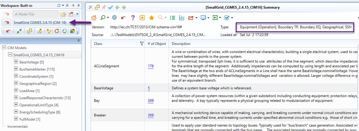
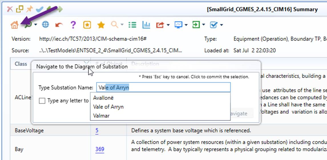
- Search for Substation “Vale of Arryn”.
- Run power flow either via context menu or by clicking the command icon, as illustrated below.
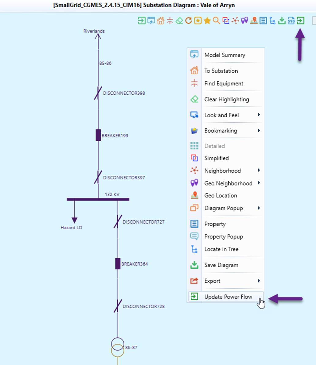
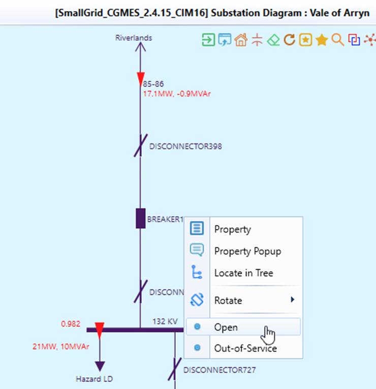
- As shown in the diagram, the 21 MW load is supplied by the grid (17 MW) and a local generator (4 MW). Can the local generator be able to pick the whole load if the supply from the grid is interrupted? To simulate this scenario, we will open BREAKER199. This can be achieved via context menu associated with the breaker symbol or label, as illustrated below.
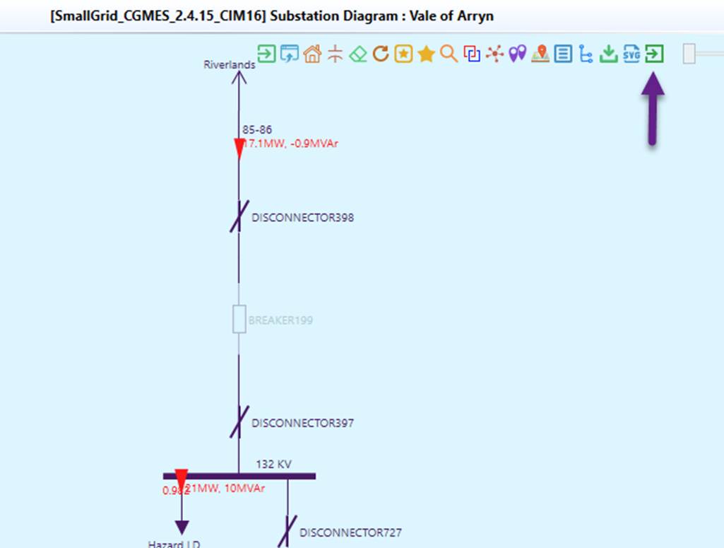
- Run power flow after the breaker is opened. Note: the Substation is now separated from the grid. There are two islands now.
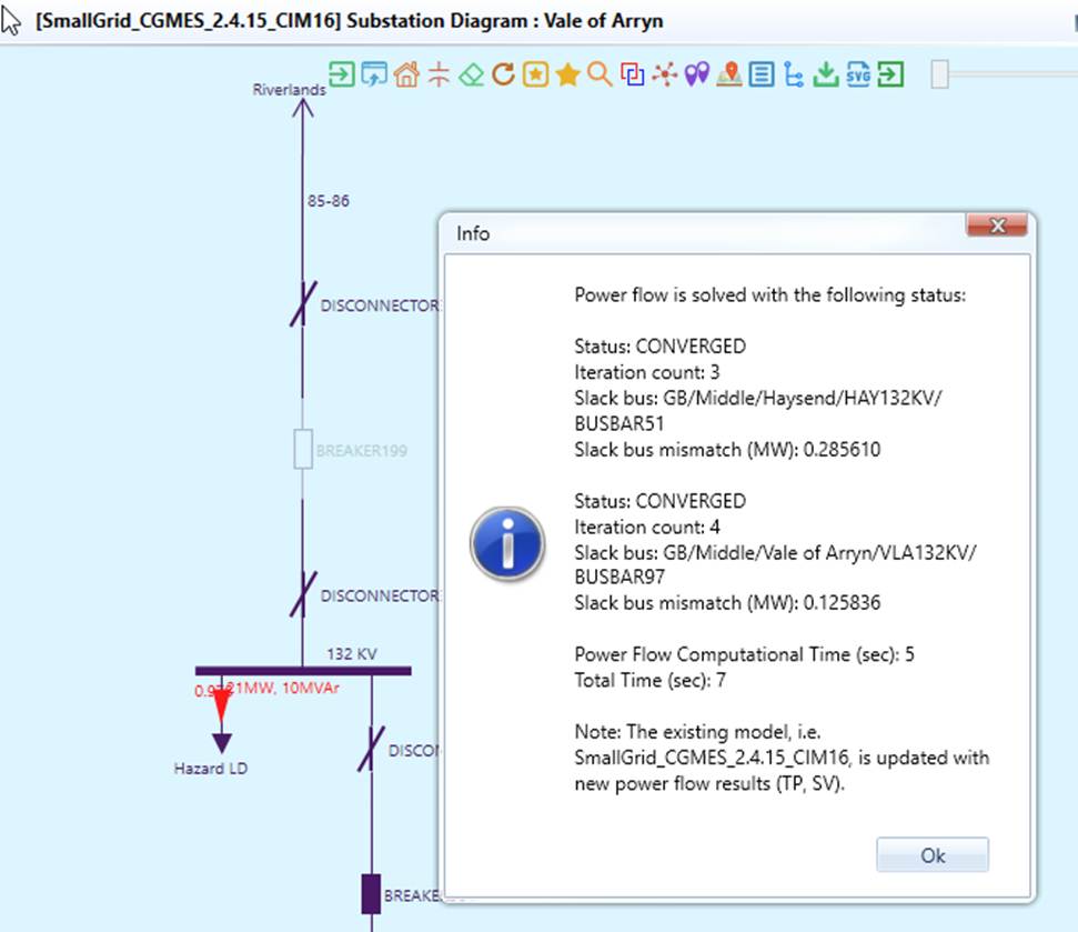
- The pop-up message shows that the power flow converges well for both islands.
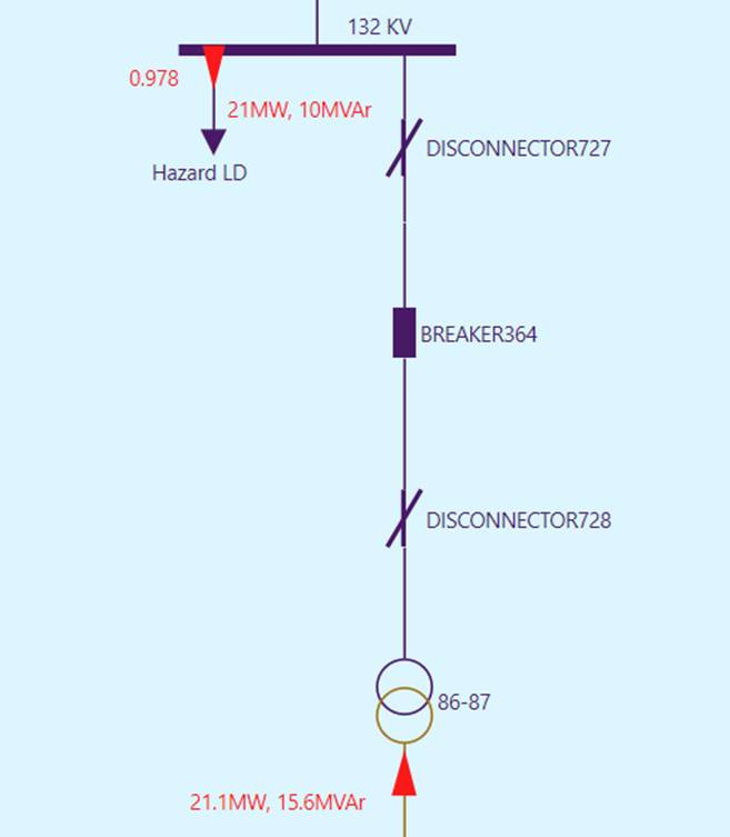
- The simulation shows that the 21 MW load is now fully picked up by the local generator.
Hands-On Lab 6: Power Flow Reporting
- Objective: To learn the basic of power flow reporting.
- Test Model: Svedala, an assembled CGMES 3.0/CIM 17 model from ENTSO-E CGMES 3.0 Test Configurations (https://www.entsoe.eu/Documents/CIM_documents/Grid_Model_CIM/TestConfigurations_packageCASv2.0.zip). This is a node/breaker model containing reality-based Substations and with power flow results published.
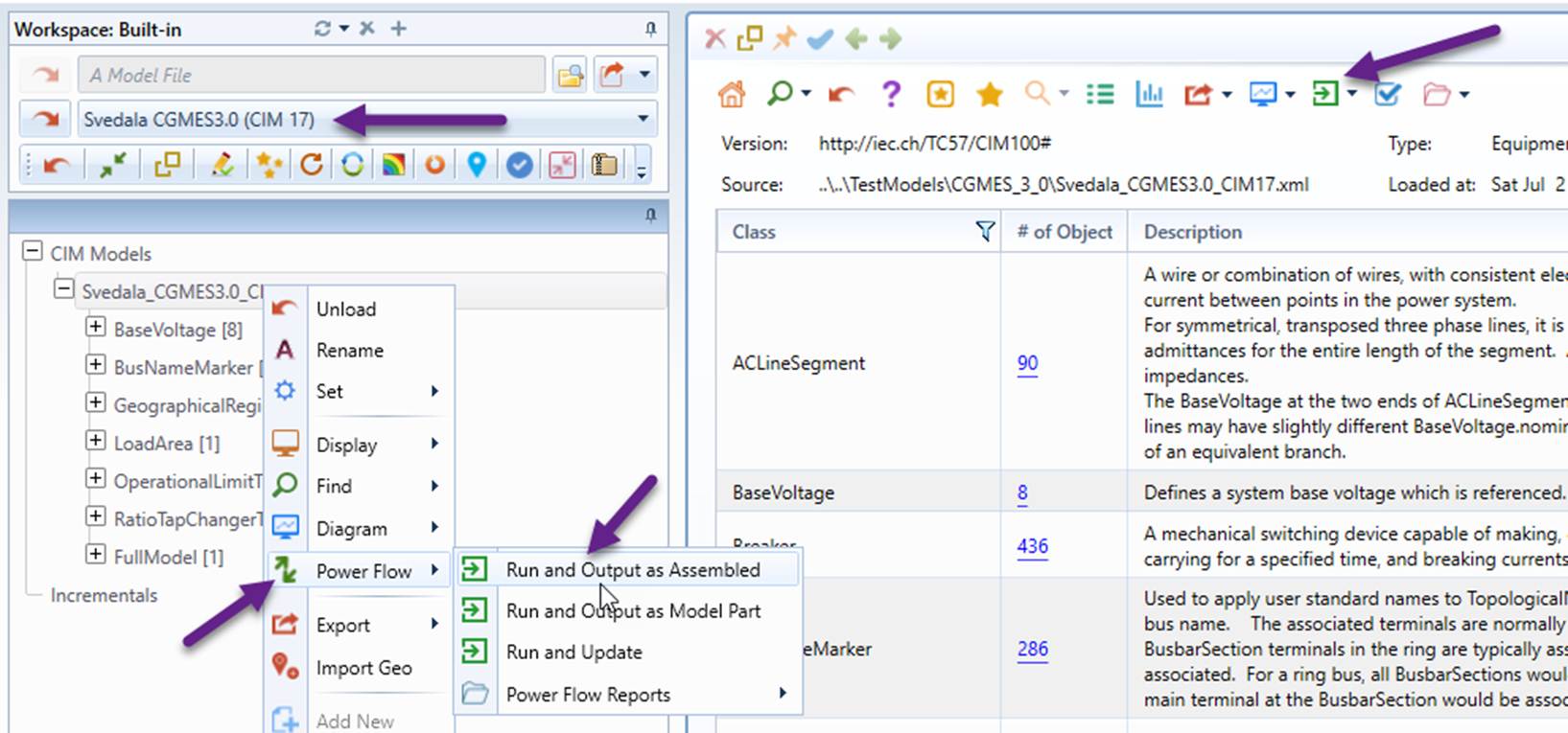
- Load “Svedala CGMES 3.0 (CIM 17)” from data source dropdown list, as illustrated.
- Invoke “Power Flow→Run and Output as Assembled” from the context menu associated with the model tree node or from the icon dropdown in the model Summary display, as illustrated
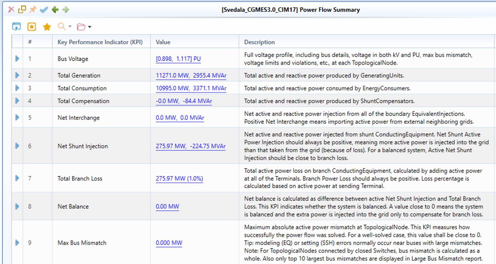
- After power flow execution is completed, a separate model is created with the Power Flow Summary Report is subsequently displayed, showing the Key Performance Indicators (KPIs) of the power flow results.
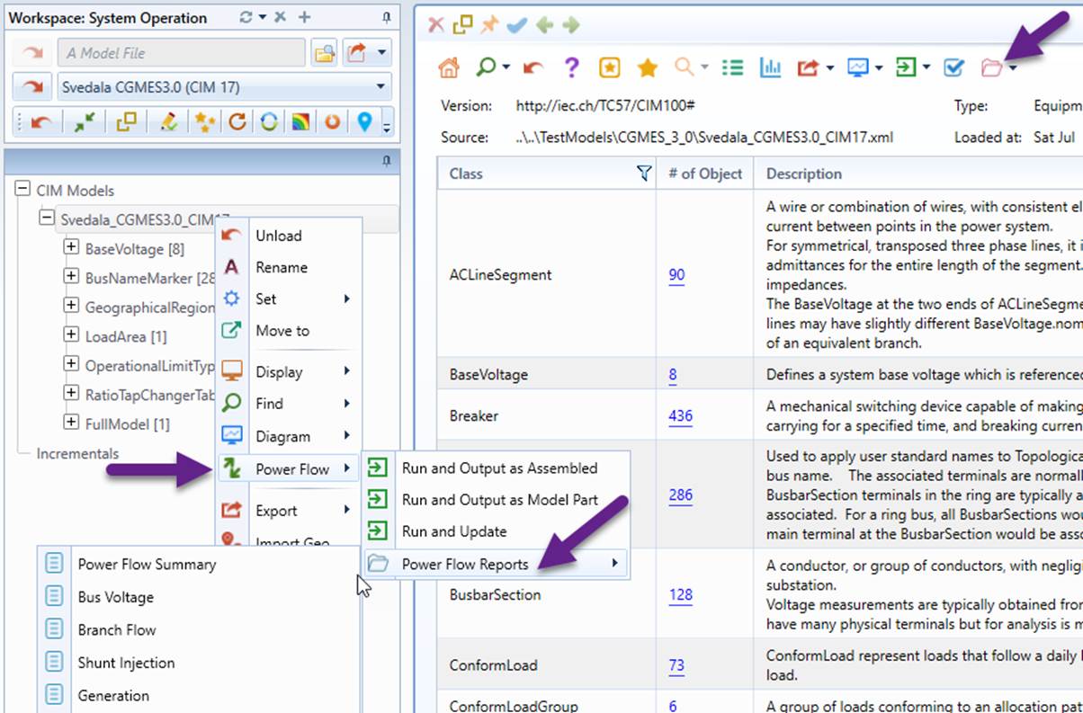
- While the detailed reports can be called from each associated KPI, the formal way to call power flow reports is via the context menu associated with model tree node, or from the dropdown icons in the Summary display of the model.
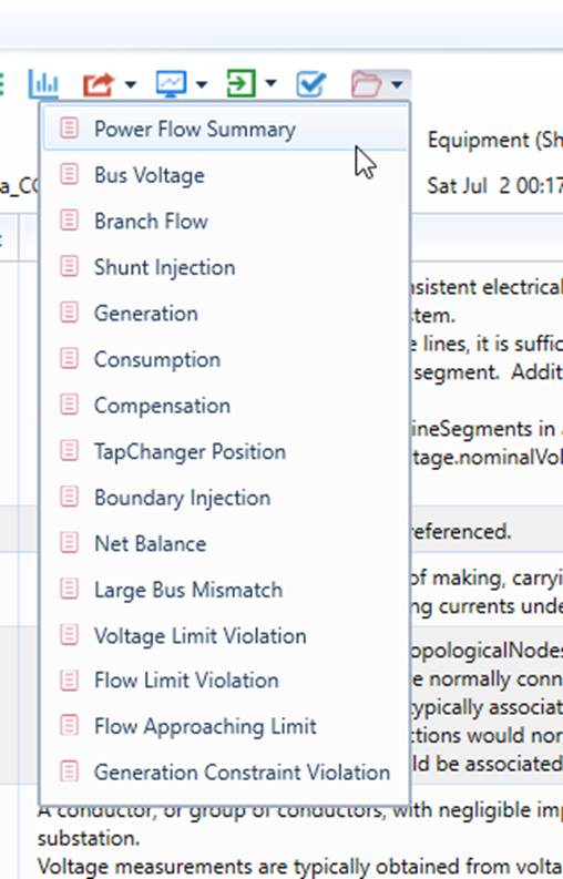
- Call detailed power flow reports, and
- Sort the report by clicking the column header;
- Click a selected Name to call the diagram, as illustrated below;
- Click a selected Path to locate the associated tree item in the navigation tree.
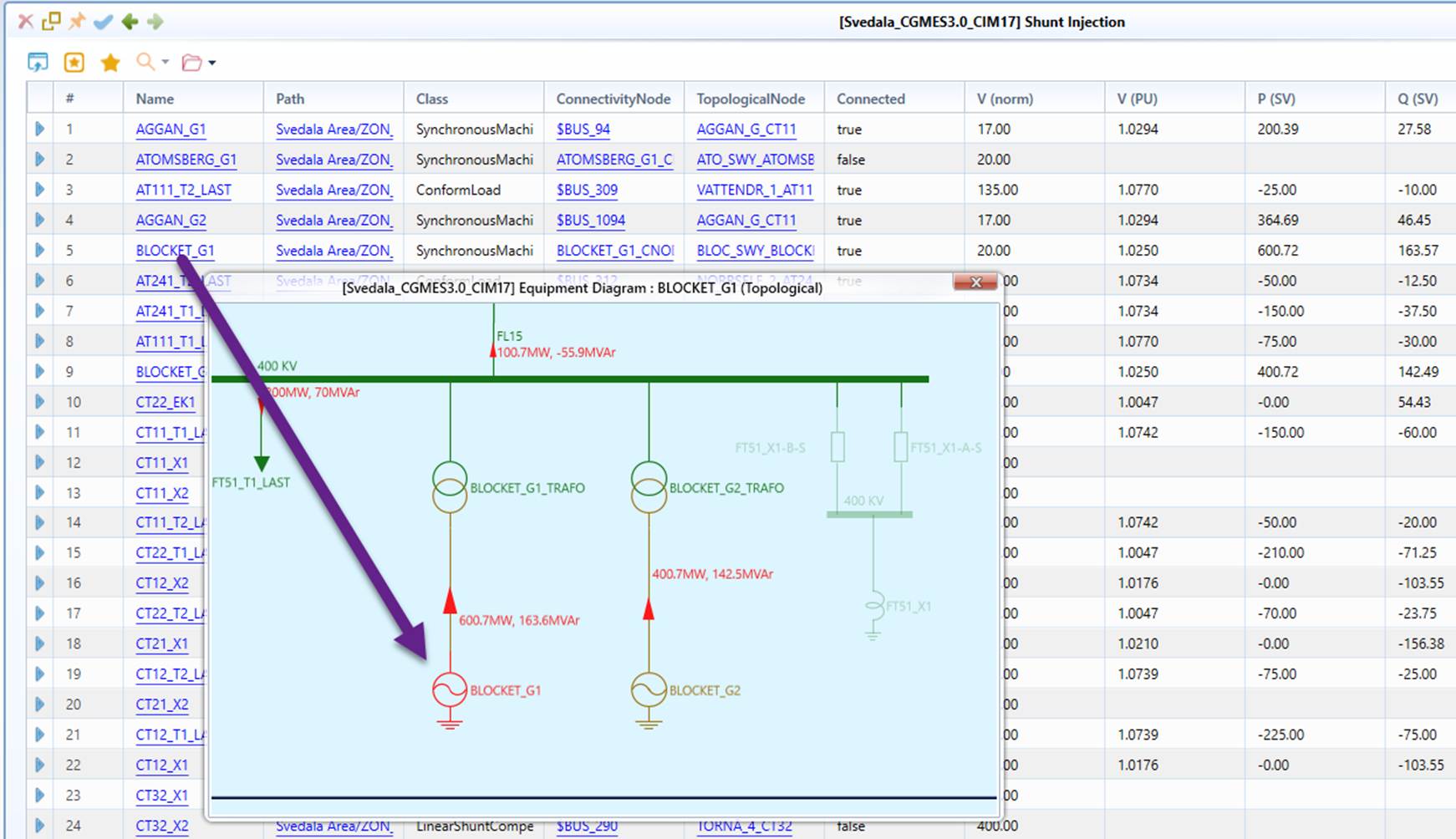
Hands-On Lab 7: Power Flow Visualization
- Objective: To learn the basic of Power Flow Visualization.
- Test Model: SmallGrid, an assembled CGMES 2..4.15/CIM 16 IGM package from ENTSO-E CGMES 2.4.15 Test Configurations (https://www.entsoe.eu/Documents/CIM_documents/Grid_Model_CIM/CGMES_v2.4.15_TestConfigurations_v4.0.3.zip). This is a node/breaker model containing all model parts of an IGM & boundary and with power flow results published. However the Topology (TP) and State Variable (SV) model parts are removed. So the assembled test model contains the minimum data set required to run power flow, i.e. Equipment (EQ) and Steady State Hypothesis (SSH) model parts.
- Load “SmallGrid CGMES 2.4.15 (CIM 16)” from data source dropdown list. Call geographical diagram from the model Summary, as illustrated below.
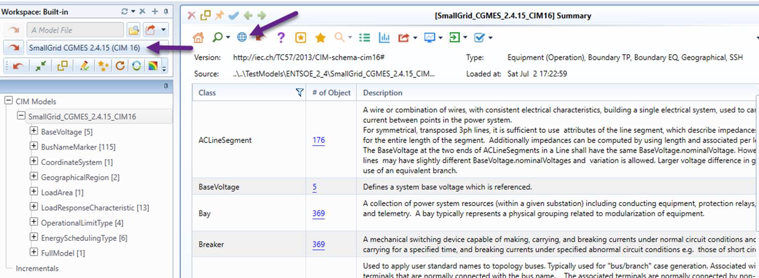
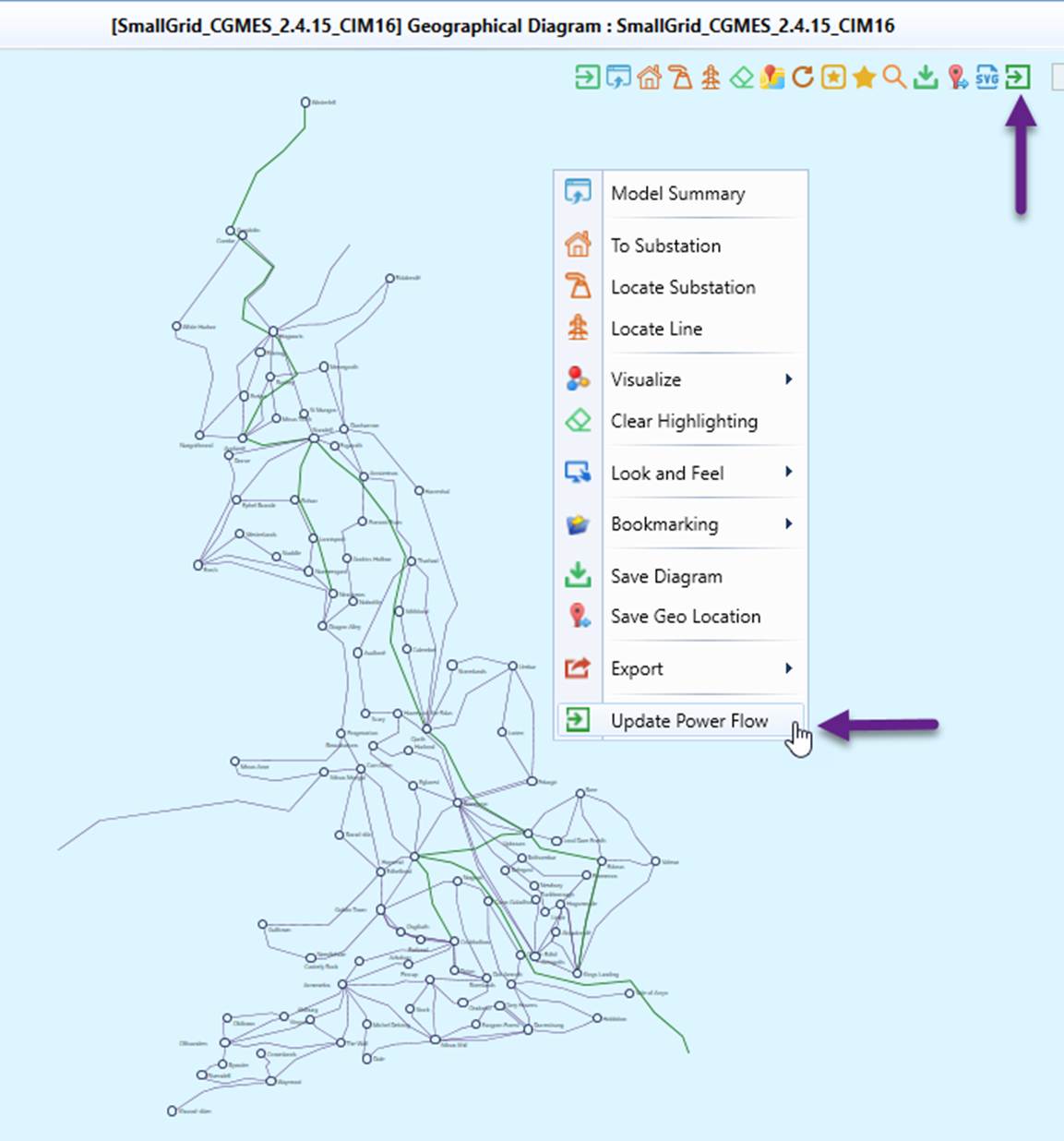
- Run Power Flow either via context menu or by clicking the command icon, as illustrated below.
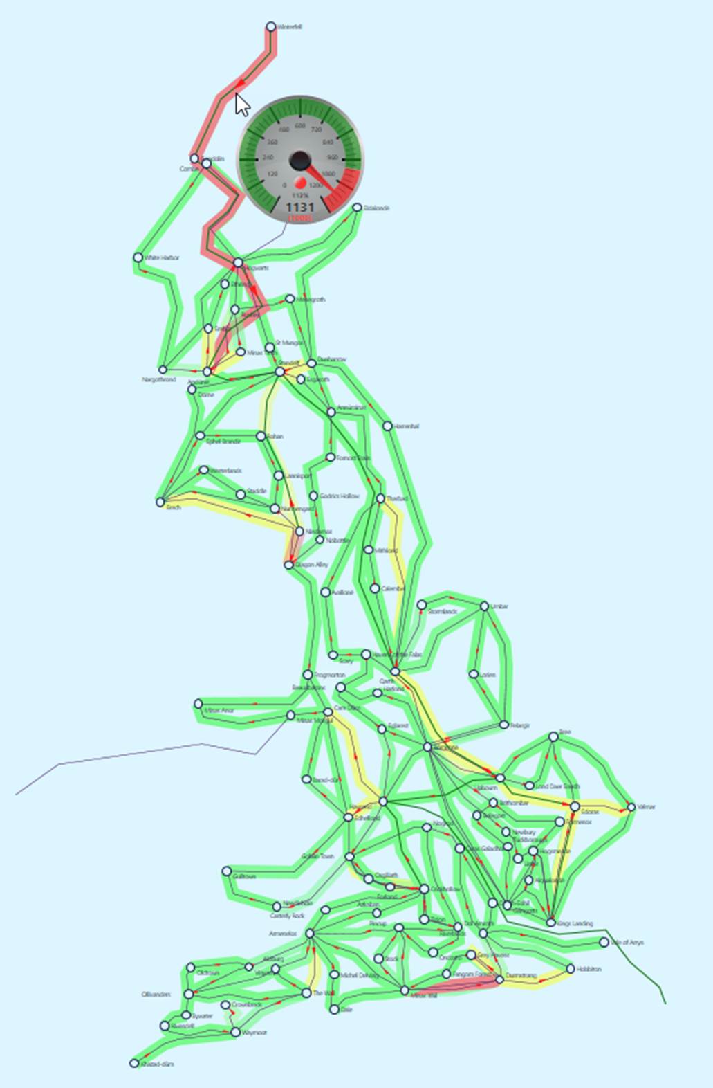
- Right-mouse-click a blank spot to invoke the diagram content menu. Invoke Visualize→Flow→Limit Profile, as illustrated.
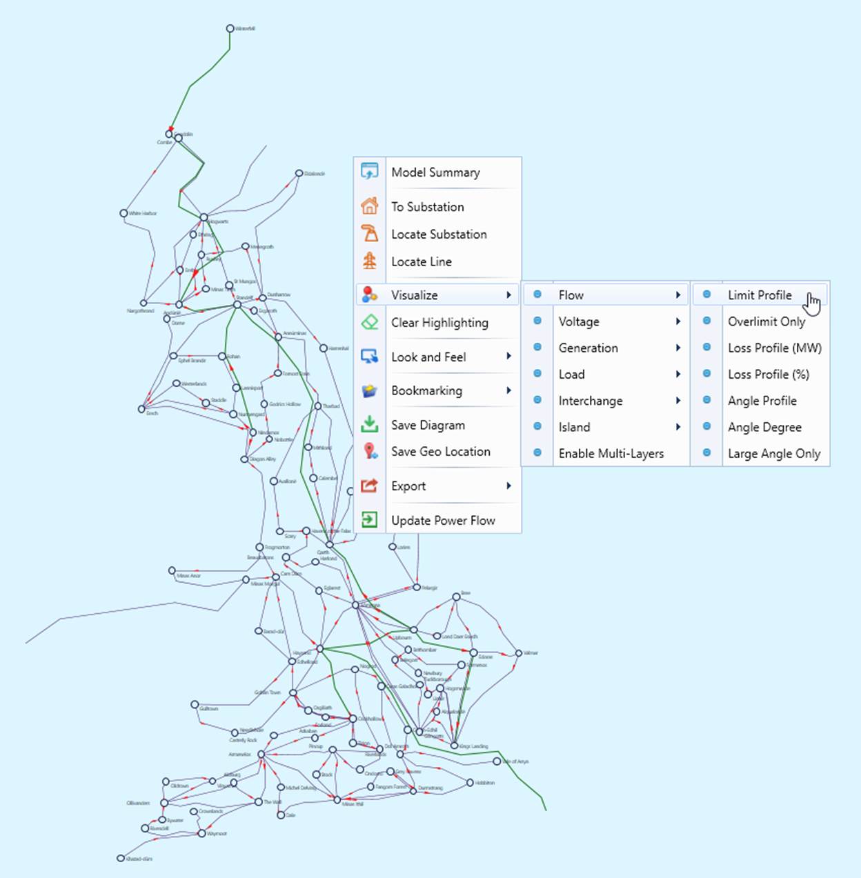
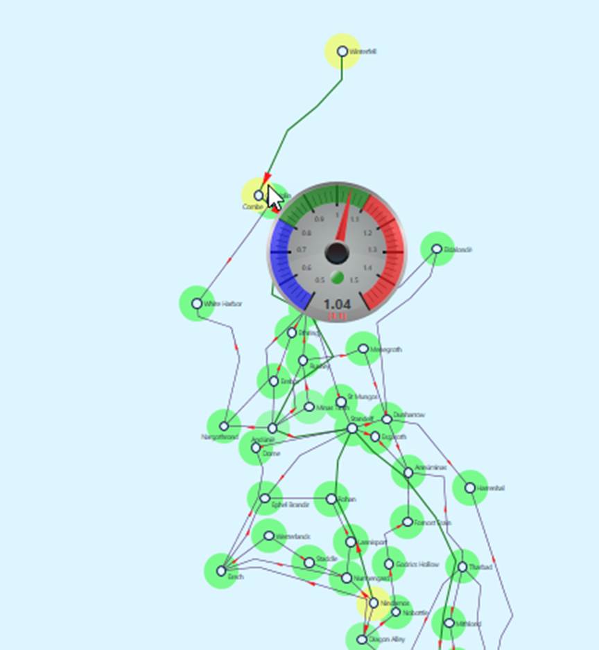
- The diagram is color-profiled, enabling users to visualize the flow limit violations. Moving the mouse to the line with limit violated, a gauge chart is popped up, showing the severity of limit violation.
- Try Visualize→Voltage→High Limit Profile and other visualizations.